9 Naive Bayes Classifier

How can we make highly accurate predictions with minimal data and computation? Imagine a bank deciding whether to approve a loan based on some factors—such as a customer’s income, age, and mortgage status. The Naive Bayes classifier offers a remarkably simple yet effective approach to such problems, relying on probability theory to make rapid, informed decisions.

Naive Bayes is a probabilistic classification algorithm that balances simplicity with effectiveness, making it a widely used approach in machine learning. It belongs to a family of classifiers based on Bayes’ theorem and operates under a key simplifying assumption: all features are conditionally independent given the target class. While this assumption is rarely true in real-world data, it allows for fast computation and efficient probability estimation, making the algorithm highly scalable and practical.

Despite its simplicity, Naive Bayes delivers strong performance in a variety of applications, particularly in text classification, spam detection, sentiment analysis, and financial risk assessment. In these domains, feature dependencies are often weak enough that the independence assumption does not significantly impact accuracy.

Beyond its theoretical foundations, Naive Bayes is computationally efficient, making it well-suited for large-scale datasets with high-dimensional feature spaces. For instance, in risk prediction, where multiple financial indicators must be analyzed, Naive Bayes can assess a customer’s likelihood of default in milliseconds. Its intuitive probabilistic reasoning and ease of implementation make it a valuable tool for both beginners and experienced practitioners.

The power of Naive Bayes comes from its foundation in Bayesian probability theory, specifically Bayes’ Theorem, introduced by the 18th-century mathematician Thomas Bayes.⁶ This theorem provides a mathematical framework for updating probability estimates as new data becomes available. By combining prior knowledge with new evidence, Bayes’ theorem serves as the basis for many Bayesian methods in statistics and machine learning.

Strengths and Limitations

The Naive Bayes classifier is widely valued for its simplicity and efficiency. It offers several advantages:

• It performs well on high-dimensional datasets, such as text classification problems with thousands of features.
  
• It is computationally efficient, making it ideal for real-time applications like spam filtering and risk prediction.
  
• It remains effective even when the independence assumption is violated, as long as feature dependencies are not too strong.

However, Naive Bayes also has limitations:

• The assumption that features are conditionally independent is rarely true in real-world datasets, especially when features exhibit strong correlations.
  
• It struggles with continuous data unless a Gaussian distribution is assumed, which may not always be appropriate.
  
• More complex models, such as decision trees or gradient boosting, often outperform Naive Bayes on datasets with intricate relationships between features.

Despite these limitations, Naive Bayes remains an essential tool in machine learning. Its ease of implementation, interpretability, and strong baseline performance make it a valuable first-choice model for many classification tasks.

What This Chapter Covers

This chapter provides a comprehensive exploration of the Naive Bayes classifier. Specifically, we will:

1. Explain the mathematical foundations of Naive Bayes, focusing on Bayes’ theorem and its role in probabilistic classification.
   
2. Walk through the mechanics of Naive Bayes with step-by-step examples.
   
3. Introduce different variants of the algorithm—Gaussian Naive Bayes, Multinomial Naive Bayes, and Bernoulli Naive Bayes—and discuss their appropriate use cases.
   
4. Examine practical considerations, including strengths, limitations, and real-world applications.
   
5. Implement Naive Bayes in R using the risk dataset from the liver package to demonstrate its effectiveness.

By the end of this chapter, you will have a thorough understanding of the Naive Bayes classifier, equipping you to apply it confidently in real-world classification problems.

9.1 Bayes’ Theorem and Probabilistic Foundations

When evaluating financial risk, how do we update our beliefs about a borrower’s likelihood of defaulting as new information—such as income, debt, or mortgage status—becomes available? The ability to quantify uncertainty and refine predictions as new evidence arises is essential in decision-making, and this is precisely what Bayes’ Theorem provides.

This theorem forms the foundation of probabilistic learning, helping us make data-driven decisions across diverse fields, including finance, medicine, and machine learning. When determining whether a loan applicant poses a financial risk, we often start with general expectations based on population statistics (prior knowledge). However, as additional details—such as mortgage status or outstanding loans—become available, this new evidence refines our estimate (posterior probability), leading to more informed decisions.

The foundation for this method was laid by Thomas Bayes, an 18th-century Presbyterian minister and self-taught mathematician. His pioneering work introduced a systematic approach to updating probabilities as new data emerges, forming the basis of what is now known as Bayesian inference. Those interested in exploring this concept further may find the book “Everything Is Predictable: How Bayesian Statistics Explain Our World” insightful. The author argues that Bayesian statistics not only help predict the future but also shape rational decision-making in everyday life.

The Essence of Bayes’ Theorem

Bayes’ Theorem provides a systematic way to update probabilities in light of new evidence. It answers the question: Given what we already know, how should our belief in a hypothesis change when we observe new data?

Mathematically, Bayes’ Theorem is expressed as:

$$\begin{array}{}P\left(A|B\right)=P\left(A\right)\cdot \frac{P\left(B|A\right)}{P\left(B\right)}& \text{(9.1)}\end{array}$$

Where:

• $P\left(A|B\right)$ is the posterior probability, representing the probability of event $A$ (hypothesis) given that event $B$ (evidence) has occurred.
  
• $P\left(A\right)$ is the prior probability, which reflects our initial belief about $A$ before considering $B$.
  
• $P\left(B|A\right)$ is the likelihood, representing the probability of observing $B$ assuming $A$ is true.
  
• $P\left(B\right)$ is the evidence, which accounts for the total probability of observing $B$.

Bayes’ Theorem provides a structured way to refine our understanding of uncertainty by combining prior knowledge with new observations. This principle underpins many probabilistic learning techniques, including the Naive Bayes classifier.

To illustrate its application, consider a financial risk assessment scenario from the risk dataset in the liver package. Suppose we want to estimate the probability that a customer has a good risk profile ($A$) given that they have a mortgage ($B$). Financial institutions often use such risk models to assess creditworthiness based on various factors, including mortgage status.

Example 9.1 Let’s use the risk dataset to calculate the probability of a customer being classified as good risk, given that they have a mortgage. We start by loading the dataset and inspecting the relevant data:

library(liver)         

data(risk)

xtabs(~ risk + mortgage, data = risk)
              mortgage
   risk        yes no
     good risk  81 42
     bad risk   94 29

To improve readability, we add row and column totals to the contingency table:

addmargins(xtabs(~ risk + mortgage, data = risk))
              mortgage
   risk        yes  no Sum
     good risk  81  42 123
     bad risk   94  29 123
     Sum       175  71 246

Now, we define the relevant events:

• $A$: The customer has a good risk profile.
  
• $B$: The customer has a mortgage (mortgage = yes).

The prior probability of a customer having good risk is given by:

$$P\left(A\right)=\frac{\text{Total Good Risk Cases}}{\text{Total Cases}}=\frac{123}{246}=0.5$$

Using Bayes’ Theorem, we compute the probability of a customer being classified as good risk given that they have a mortgage:

$$\begin{array}{cc}P\left(\text{Good Risk}|\text{Mortgage = Yes}\right)& =\frac{P(\text{Good Risk}\cap \text{Mortgage = Yes})}{P\left(\text{Mortgage = Yes}\right)}\\ & =\frac{\text{Good Risk with Mortgage Cases}}{\text{Total Mortgage Cases}}\\ & =\frac{81}{175}\\ & =0.463\end{array}$$

This result indicates that among customers with mortgages, the probability of having a good risk profile is lower than in the general population. Such insights help financial institutions refine credit risk models by incorporating new evidence systematically.

How Does Bayes’ Theorem Work?

Bayes’ Theorem provides a structured way to update our understanding of uncertainty based on new information. In many real-world scenarios, we start with an initial belief about an event’s likelihood, and as we gather more data, we refine this belief to make better-informed decisions.

For instance, in financial risk assessment, banks initially estimate a borrower’s risk level based on general population statistics. However, as they collect more details—such as income, credit history, and mortgage status—Bayes’ Theorem allows them to update the probability of the borrower being classified as high or low risk. This enables more precise lending decisions.

Beyond finance, Bayes’ Theorem is widely applied in other domains:

• In medical diagnostics, it helps estimate the probability of a disease ($A$) given a positive test result ($B$), incorporating both the test’s reliability and the disease’s prevalence.
  
• In spam detection, it computes the probability that an email is spam ($A$) based on the presence of certain keywords ($B$), refining predictions as new messages are analyzed.

Probability theory provides a rigorous mathematical structure for reasoning under uncertainty. Bayes’ Theorem extends this by enabling a systematic approach to learning from data and improving decision-making in fields ranging from healthcare to finance and beyond.

A Gateway to Naive Bayes

Bayes’ Theorem provides a mathematical foundation for updating probabilities as new evidence emerges. However, in practical classification tasks, computing these probabilities directly can be computationally expensive, particularly for datasets with many features. This is where the Naive Bayes Classifier comes in.

Naive Bayes builds directly on Bayes’ Theorem by introducing a key simplification: it assumes that features are conditionally independent given the target class. While this assumption is rarely true in real-world data, it drastically reduces computational complexity, making the algorithm highly efficient for large-scale problems.

Despite this simplification, Naive Bayes performs remarkably well in many applications. For example, in financial risk prediction, a bank may assess a borrower’s creditworthiness using features like income, loan history, and mortgage status. While these factors may be correlated, Naive Bayes assumes they are independent given the borrower’s risk category, allowing for rapid probability estimation and classification.

This efficiency makes Naive Bayes particularly effective in domains such as text classification, spam filtering, and sentiment analysis, where feature independence is a reasonable approximation. In the following sections, we will explore how this assumption enables fast, interpretable, and scalable classification while maintaining competitive performance.

9.2 Why is it Called “Naive”?

Imagine assessing a borrower’s financial risk based on their income, mortgage status, and number of loans. Intuitively, these factors are related—individuals with higher income may have better loan repayment histories, and those with more loans might have a higher probability of financial distress. However, Naive Bayes assumes that all these features are independent once we know the risk category (good risk or bad risk).

This assumption is what makes the algorithm “naive.” In reality, features are often correlated, such as income and age, but by treating them as independent, Naive Bayes significantly simplifies probability calculations, making it both efficient and scalable.

To illustrate, consider the risk dataset from the liver package:

str(risk)
   'data.frame':    246 obs. of  6 variables:
    $ age     : int  34 37 29 33 39 28 28 25 41 26 ...
    $ marital : Factor w/ 3 levels "single","married",..: 3 3 3 3 3 3 3 3 3 3 ...
    $ income  : num  28061 28009 27615 27287 26954 ...
    $ mortgage: Factor w/ 2 levels "yes","no": 1 2 2 1 1 2 2 2 2 2 ...
    $ nr.loans: int  3 2 2 2 2 2 3 2 2 2 ...
    $ risk    : Factor w/ 2 levels "good risk","bad risk": 2 2 2 2 2 2 2 2 2 2 ...

This dataset includes financial indicators such as age, income, marital status, mortgage, and number of loans. Naive Bayes assumes that given a person’s risk classification (good risk or bad risk), these features do not influence one another. Mathematically, the probability of a customer being in the good risk category given their attributes is expressed as:

$$P(Y=y_1|X_1,X_2,\dots ,X_5)=\frac{P(Y=y_1)\cdot P(X_1,X_2,\dots ,X_5|Y=y_1)}{P(X_1,X_2,\dots ,X_5)}$$

However, directly computing $P(X_1,X_2,\dots ,X_5|Y=y_1)$ is computationally expensive, especially as the number of features grows. For instance, in datasets with hundreds or thousands of features, storing and calculating joint probabilities for all possible feature combinations becomes impractical.

The naive assumption of conditional independence simplifies this problem by expressing the joint probability as the product of individual probabilities:

$$P(X_1,X_2,\dots ,X_5|Y=y_1)=P(X_1|Y=y_1)\cdot P(X_2|Y=y_1)\cdots P(X_5|Y=y_1)$$

This transformation eliminates the need to compute complex joint probabilities, making the algorithm scalable even for high-dimensional data. Instead of handling an exponential number of feature combinations, Naive Bayes only requires computing simple conditional probabilities for each feature given the class label.

In practice, this independence assumption is rarely true—features often exhibit some degree of correlation. However, Naive Bayes frequently performs well despite this limitation. It remains widely used in domains where:

• Feature dependencies are weak enough that the assumption does not significantly impact accuracy.
• The focus is on speed and interpretability rather than capturing complex relationships.
• Slight violations of the independence assumption do not severely affect predictive performance.

For example, in risk prediction, while income and mortgage status are likely correlated, treating them as independent still allows Naive Bayes to classify borrowers effectively. Similarly, in spam detection or text classification, where features (such as words in an email) are often independent enough, the algorithm delivers fast and accurate predictions.

By balancing computational efficiency with predictive power, Naive Bayes remains a foundational algorithm in machine learning, particularly for applications that demand scalability and interpretability.

9.3 The Laplace Smoothing Technique

One of the challenges in Naive Bayes classification is handling feature categories that appear in the test data but are absent in the training data. Suppose we train a model on a dataset where no borrowers classified as “bad risk” are married. If we later encounter a married borrower in the test set, Naive Bayes would compute $P\left(\text{bad risk}|\text{married}\right)$ as zero. Because the algorithm multiplies probabilities when making predictions, even a single zero probability results in an overall probability of zero for that class, making it impossible for the model to predict that class.

This issue arises because Naive Bayes estimates probabilities from frequency counts in the training data. If a feature value never appears in a given class, its estimated probability is zero, which can lead to misclassification errors. To address this, Laplace smoothing (also known as add-one smoothing) is used. Named after the mathematician Pierre-Simon Laplace, this technique ensures that every feature-category combination has a small, non-zero probability, even if it is missing in the training data.

To illustrate, consider the marital variable in the risk dataset. Suppose the category married is entirely absent for customers labeled as bad risk. This scenario can be visualized as follows:

            risk
   marital   good risk bad risk
     single         21       11
     married        51        0
     other           8       10

Without smoothing, the probability of bad risk given married is:

$$P\left(\text{bad risk}|\text{married}\right)=\frac{\text{count}(\text{bad risk}\cap \text{married})}{\text{count}\left(\text{married}\right)}=\frac{0}{\text{count}\left(\text{married}\right)}=0$$

This means that any married borrower will always be classified as good risk, regardless of their other characteristics.

Laplace smoothing resolves this by modifying the probability calculation. Instead of assigning a strict zero probability, a small constant $k$ (usually $k=1$) is added to each count in the frequency table. The adjusted probability is given by:

$$P\left(\text{bad risk}|\text{married}\right)=\frac{\text{count}(\text{bad risk}\cap \text{married})+k}{\text{count}\left(\text{bad risk}\right)+k\times \text{number of categories in}\text{marital}}$$

This adjustment ensures that: - Every category receives a small positive count, avoiding zero probabilities. - The total probability distribution remains valid.

In R, Laplace smoothing can be applied using the laplace argument in the naivebayes package. By default, laplace = 0, meaning no smoothing is applied. To apply smoothing, simply set laplace = 1:

library(naivebayes)

# Fit Naive Bayes with Laplace smoothing
formula_nb = risk ~ age + income + marital + mortgage + nr.loans

model <- naive_bayes(formula = formula_nb, data = risk, laplace = 1)

This ensures that no category is assigned a probability of zero, improving the model’s robustness—particularly in cases where the training data is limited or imbalanced.

Laplace smoothing is a simple yet effective technique that prevents Naive Bayes from being overly sensitive to missing categories in training data. While $k=1$ is the most common approach, the value of $k$ can be adjusted based on specific domain knowledge. By ensuring that probabilities remain well-defined, Laplace smoothing enhances the reliability of Naive Bayes classifiers in real-world applications.

9.4 Types of Naive Bayes Classifiers

Naive Bayes is a versatile algorithm with different variants designed for specific data types and distributions. The choice of which variant to use depends on the nature of the features and the assumptions made about their underlying distribution. The three most common types are:

• Multinomial Naive Bayes: Best suited for categorical or count-based features, such as word frequencies in text data. This variant is commonly used in text classification, where features represent discrete counts (e.g., the number of times a word appears in a document). In the risk dataset, the marital variable, which takes categorical values such as single, married, and other, aligns well with this variant.

• Bernoulli Naive Bayes: Designed for binary features, where each variable represents the presence or absence of a characteristic. This variant is particularly useful in applications where data is represented as a set of binary indicators, such as whether an email contains a specific keyword in spam detection. In the risk dataset, the mortgage variable, which has two possible values (yes or no), is an example of a binary feature suitable for this approach.

• Gaussian Naive Bayes: Applied to continuous data where features are assumed to follow a normal (Gaussian) distribution. This variant estimates the likelihood of each feature using a normal distribution, making it ideal for datasets with numerical attributes such as age, income, or credit scores. In the risk dataset, variables like age and income are continuous and thus well suited for this variant.

Each of these Naive Bayes classifiers is optimized for different data types, making it essential to select the one that best fits the dataset’s characteristics. Understanding these distinctions allows for better model selection and improved performance. In the following sections, we will explore each variant in greater detail, examining their assumptions, strengths, and use cases.

9.5 Case Study: Predicting Financial Risk with Naive Bayes

Financial institutions must assess loan applicants carefully to balance profitability with risk management. Lending decisions rely on estimating the likelihood of default, which depends on various financial and demographic factors. A robust risk classification model helps institutions make informed decisions, reducing financial losses while ensuring fair lending practices.

In this case study, we apply the Naive Bayes classifier to predict whether a customer is a good risk or bad risk based on financial and demographic attributes. Using the risk dataset from the liver package in R, we train and evaluate a probabilistic classification model. This case study demonstrates how Naive Bayes can be leveraged in financial decision-making, providing insights into customer risk profiles and supporting more effective credit evaluation.

Problem Understanding

A key challenge in financial risk assessment is distinguishing between customers who are likely to repay loans and those at higher risk of default. Predictive modeling enables financial institutions to anticipate risk, optimize credit policies, and reduce non-performing loans. Key business questions include:

• What financial and demographic factors contribute to a customer’s risk profile?
  
• How can we predict whether a customer is a good or bad risk before approving a loan?
  
• What insights can be gained to refine lending policies and mitigate financial losses?

By analyzing the risk dataset, we aim to develop a model that classifies customers based on risk level. This will allow lenders to make data-driven decisions, improve credit scoring, and enhance loan approval strategies.

Data Understanding

The risk dataset contains financial and demographic attributes that help assess a customer’s likelihood of being classified as either a good risk or bad risk. This dataset, included in the liver package, consists of 246 observations and 6 variables. It provides a structured way to analyze customer characteristics and predict financial risk levels.

The dataset includes 5 predictors and a binary target variable, risk, which distinguishes between customers who are more or less likely to default. The key variables are:

• age: Customer’s age in years.
  
• marital: Marital status (single, married, other).
  
• income: Annual income.
  
• mortgage: Indicates whether the customer has a mortgage (yes, no).
  
• nr_loans: Number of loans held by the customer.
  
• risk: The target variable (good risk, bad risk).

For additional details about the dataset, refer to its documentation.

To begin the analysis, we load the dataset and examine its structure to understand its variables and data types:

data(risk)

str(risk)
   'data.frame':    246 obs. of  6 variables:
    $ age     : int  34 37 29 33 39 28 28 25 41 26 ...
    $ marital : Factor w/ 3 levels "single","married",..: 3 3 3 3 3 3 3 3 3 3 ...
    $ income  : num  28061 28009 27615 27287 26954 ...
    $ mortgage: Factor w/ 2 levels "yes","no": 1 2 2 1 1 2 2 2 2 2 ...
    $ nr.loans: int  3 2 2 2 2 2 3 2 2 2 ...
    $ risk    : Factor w/ 2 levels "good risk","bad risk": 2 2 2 2 2 2 2 2 2 2 ...

To gain further insights, we summarize the dataset’s key statistics:

summary(risk)
         age           marital        income      mortgage     nr.loans    
    Min.   :17.00   single :111   Min.   :15301   yes:175   Min.   :0.000  
    1st Qu.:32.00   married: 78   1st Qu.:26882   no : 71   1st Qu.:1.000  
    Median :41.00   other  : 57   Median :37662             Median :1.000  
    Mean   :40.64                 Mean   :38790             Mean   :1.309  
    3rd Qu.:50.00                 3rd Qu.:49398             3rd Qu.:2.000  
    Max.   :66.00                 Max.   :78399             Max.   :3.000  
           risk    
    good risk:123  
    bad risk :123  
                   
                   
                   
   

This summary provides an overview of variable distributions and identifies any missing values or potential anomalies. Since the dataset appears clean and well-structured, we can proceed to data preparation before training the Naive Bayes classifier.

Preparing Data for Modeling

Before training the Naive Bayes classifier, we need to split the dataset into training and testing sets. This step ensures that we can evaluate how well the model generalizes to unseen data. We use an 80/20 split, allocating 80% of the data for training and 20% for testing. To maintain consistency with previous chapters, we apply the partition() function from the liver package:

set.seed(5)

data_sets = partition(data = risk, ratio = c(0.8, 0.2))

train_set = data_sets$part1
test_set  = data_sets$part2

test_labels = test_set$risk

Setting set.seed(5) ensures reproducibility so that the same partitioning is achieved each time the code is run. The train_set will be used to train the Naive Bayes classifier, while the test_set will serve as unseen data to evaluate the model’s predictions. The test_labels vector contains the true class labels for the test set, which we will compare against the model’s predictions.

To verify that the training and test sets are representative of the original dataset, we compare the proportions of the marital variable across both sets. A chi-squared test is used to check whether the distribution of marital statuses (single, married, and other) is statistically similar between the training and test sets:

chisq.test(x = table(train_set$marital), y = table(test_set$marital))
   
    Pearson's Chi-squared test
   
   data:  table(train_set$marital) and table(test_set$marital)
   X-squared = 6, df = 4, p-value = 0.1991

This statistical test evaluates whether the proportions of marital categories differ significantly between the training and test sets. The hypotheses for the test are:
$$\{\begin{array}{c}{H}_0:\text{The proportions of marital categories are the same in both sets.}\\ H_a:\text{At least one of the proportions is different.}\end{array}$$ Since the p-value exceeds $\alpha =0.05$, we fail to reject $H_0$, meaning that the marital status distribution remains statistically similar between the training and test sets. This confirms that the partitioning process maintains the dataset’s characteristics, allowing for reliable model evaluation.

With a well-structured dataset and a validated partitioning process, we are now ready to train the Naive Bayes classifier and assess its predictive capabilities.

Applying the Naive Bayes Classifier

With the dataset partitioned and validated, we now proceed to train and evaluate the Naive Bayes classifier. The objective is to build a model using the training set and assess its ability to classify customers as good risk or bad risk in the test set.

Several R packages provide implementations of Naive Bayes, with two commonly used options being naivebayes and e1071. In this case study, we use the naivebayes package, which offers an efficient implementation of the classifier. The naive_bayes() function in this package supports various probability distributions depending on the nature of the features:

• Categorical distribution for discrete variables such as marital and mortgage.
  
• Bernoulli distribution for binary features, a special case of the categorical distribution.
  
• Poisson distribution for count-based variables, such as the number of loans.
  
• Gaussian distribution for continuous features, such as age and income.
  
• Non-parametric density estimation for continuous features when no specific distribution is assumed.

Unlike the k-NN algorithm in the previous chapter, which classifies new data without an explicit training phase, Naive Bayes follows a two-step process:

1. Training phase – The model learns probability distributions from the training data.
   
2. Prediction phase – The trained model is used to classify new data points based on the learned probabilities.

To train the model, we define a formula where risk is the target variable, and all other features serve as predictors:

formula = risk ~ age + income + mortgage + nr.loans + marital

We then apply the naive_bayes() function from the naivebayes package to train the classifier on the training dataset:

library(naivebayes)

naive_bayes = naive_bayes(formula, data = train_set)

naive_bayes
   
   ================================= Naive Bayes ==================================
   
   Call:
   naive_bayes.formula(formula = formula, data = train_set)
   
   -------------------------------------------------------------------------------- 
    
   Laplace smoothing: 0
   
   -------------------------------------------------------------------------------- 
    
   A priori probabilities: 
   
   good risk  bad risk 
   0.4923858 0.5076142 
   
   -------------------------------------------------------------------------------- 
    
   Tables: 
   
   -------------------------------------------------------------------------------- 
   :: age (Gaussian) 
   -------------------------------------------------------------------------------- 
         
   age    good risk  bad risk
     mean 46.453608 35.470000
     sd    8.563513  9.542520
   
   -------------------------------------------------------------------------------- 
   :: income (Gaussian) 
   -------------------------------------------------------------------------------- 
         
   income good risk  bad risk
     mean 48888.987 27309.560
     sd    9986.962  7534.639
   
   -------------------------------------------------------------------------------- 
   :: mortgage (Bernoulli) 
   -------------------------------------------------------------------------------- 
           
   mortgage good risk  bad risk
        yes 0.6804124 0.7400000
        no  0.3195876 0.2600000
   
   -------------------------------------------------------------------------------- 
   :: nr.loans (Gaussian) 
   -------------------------------------------------------------------------------- 
           
   nr.loans good risk  bad risk
       mean 1.0309278 1.6600000
       sd   0.7282057 0.7550503
   
   -------------------------------------------------------------------------------- 
   :: marital (Categorical) 
   -------------------------------------------------------------------------------- 
            
   marital    good risk   bad risk
     single  0.38144330 0.49000000
     married 0.52577320 0.11000000
     other   0.09278351 0.40000000
   
   --------------------------------------------------------------------------------

The naive_bayes() function estimates the probability distributions for each feature, conditioned on the target class. Specifically:

• Categorical features (e.g., marital, mortgage) – The function computes class-conditional probabilities.
  
• Continuous features (e.g., age, income, nr.loans) – The function assumes a Gaussian distribution and calculates the mean and standard deviation for each class.

To inspect the model’s learned probability distributions, we summarize the trained model:

summary(naive_bayes)
   
   ================================= Naive Bayes ================================== 
    
   - Call: naive_bayes.formula(formula = formula, data = train_set) 
   - Laplace: 0 
   - Classes: 2 
   - Samples: 197 
   - Features: 5 
   - Conditional distributions: 
       - Bernoulli: 1
       - Categorical: 1
       - Gaussian: 3
   - Prior probabilities: 
       - good risk: 0.4924
       - bad risk: 0.5076
   
   --------------------------------------------------------------------------------

The summary output provides useful insights into how the classifier models each feature’s probability distribution. This forms the basis for making predictions on new data points, which we explore in the next section.

Prediction and Model Evaluation

After training the Naive Bayes classifier, we evaluate its performance by applying it to the test set, which contains customers unseen during training. The goal is to compare the predicted probabilities with the actual class labels stored in test_labels.

To obtain the predicted class probabilities, we use the predict() function from the naivebayes package:

prob_naive_bayes = predict(naive_bayes, test_set, type = "prob")

By specifying type = "prob", the function returns posterior probabilities for each class instead of discrete predictions.

To inspect the model’s predictions, we display the first 10 probability estimates:

# Display the first 10 predictions
round(head(prob_naive_bayes, n = 10), 3)
         good risk bad risk
    [1,]     0.001    0.999
    [2,]     0.013    0.987
    [3,]     0.000    1.000
    [4,]     0.184    0.816
    [5,]     0.614    0.386
    [6,]     0.193    0.807
    [7,]     0.002    0.998
    [8,]     0.002    0.998
    [9,]     0.378    0.622
   [10,]     0.283    0.717

The output contains two columns:

• The first column represents the probability that a customer is classified as “good risk.”
• The second column represents the probability that a customer is classified as “bad risk.”
  For example, if the second row has a probability of 0.987 for “bad risk,” it indicates that the second customer in the test set is predicted to belong to the “bad risk” category with a probability of 0.987.

This probability-based output provides flexibility in decision-making. Instead of using a fixed threshold of 0.5, financial institutions can adjust the cutoff based on business objectives. For instance, if minimizing loan defaults is the priority, a more conservative threshold may be set. In the next section, we convert these probabilities into class predictions and evaluate the model using a confusion matrix and other performance metrics.

Confusion Matrix

To assess the classification performance of our Naive Bayes model, we compute the confusion matrix using the conf.mat() and conf.mat.plot() functions from the liver package. The confusion matrix compares the predicted class probabilities with the actual class labels, allowing us to measure the model’s accuracy and analyze different types of errors.

# Extract probability of "good risk"
prob_naive_bayes = prob_naive_bayes[, 1] 

conf.mat(prob_naive_bayes, test_labels, cutoff = 0.5, reference = "good risk")
              Actual
   Predict     good risk bad risk
     good risk        24        3
     bad risk          2       20

conf.mat.plot(prob_naive_bayes, test_labels, cutoff = 0.5, reference = "good risk")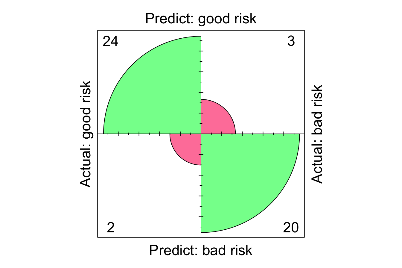

In this evaluation, we apply a classification threshold of 0.5, meaning that if a customer’s predicted probability of being a “good risk” is at least 50%, the model classifies them as “good risk”; otherwise, they are classified as “bad risk.” Additionally, we specify “good risk” as the reference class, meaning that performance metrics such as sensitivity and precision will be calculated with respect to this category.

The confusion matrix provides the following breakdown of model predictions:

• True Positives (TP): Customers correctly classified as “good risk.”
  
• True Negatives (TN): Customers correctly classified as “bad risk.”
  
• False Positives (FP): Customers incorrectly classified as “good risk” when they were actually “bad risk.”
  
• False Negatives (FN): Customers incorrectly classified as “bad risk” when they were actually “good risk.”

The values in the confusion matrix quantify the model’s classification accuracy and error rates at a cutoff of 0.5. Specifically, the model correctly predicts “24 + 20” cases and misclassifies “3 + 2” cases.

This matrix offers a structured way to assess classification performance, helping us understand how well the model differentiates between high- and low-risk customers. In the next section, we further analyze performance using additional evaluation metrics.

ROC Curve and AUC

To further evaluate the model, we compute the Receiver Operating Characteristic (ROC) curve and the Area Under the Curve (AUC) value. These metrics provide a comprehensive assessment of the model’s ability to distinguish between “good risk” and “bad risk” customers across different classification thresholds. The pROC package in R facilitates both calculations.

library(pROC)          

roc_naive_bayes = roc(test_labels, prob_naive_bayes)

ggroc(roc_naive_bayes)

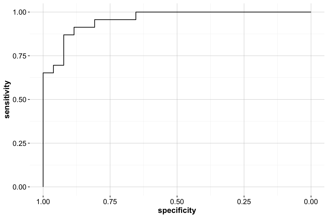
The ROC curve plots the true positive rate (sensitivity) against the false positive rate (1 - specificity) at various threshold values. A curve that remains closer to the top-left corner indicates a well-performing model, while a curve near the diagonal suggests performance close to random guessing.

Next, we compute the AUC value, which summarizes the ROC curve into a single number:

round(auc(roc_naive_bayes), 3)
   [1] 0.957

The AUC value, 0.957, represents the probability that a randomly selected “good risk” customer will receive a higher predicted probability than a randomly selected “bad risk” customer. An AUC closer to 1 indicates strong predictive performance, while an AUC of 0.5 suggests no better performance than random guessing.

By analyzing the ROC curve and AUC, financial institutions can adjust the decision threshold to align with business objectives. If minimizing false negatives (misclassifying high-risk customers as low-risk) is a priority, the threshold can be lowered to increase sensitivity. Conversely, if false positives (denying loans to eligible customers) are a concern, a higher threshold can be set to improve specificity.

Through this case study, we have demonstrated how Naive Bayes can be applied to financial risk assessment. By evaluating model performance using the confusion matrix, ROC curve, and AUC, we identified its strengths and limitations. This highlights the efficiency and interpretability of Naive Bayes, making it a valuable tool for probabilistic classification in financial decision-making.

Takeaways from the Case Study

This case study demonstrated how Naive Bayes can be applied to financial risk assessment by classifying customers as either good risk or bad risk based on demographic and financial attributes. Through key evaluation metrics such as the confusion matrix, ROC curve, and AUC, we analyzed the model’s predictive power and identified its strengths and limitations.

The results highlight the efficiency, simplicity, and interpretability of Naive Bayes, making it a valuable tool for probabilistic classification in financial decision-making. The model’s ability to provide probability estimates allows institutions to adjust decision thresholds based on business priorities—whether prioritizing sensitivity to minimize high-risk approvals or improving specificity to reduce false rejections.

While Naive Bayes performs well in this scenario, it relies on the assumption of feature independence, which may not always hold in real-world financial data. Future improvements could include using ensemble models or integrating additional financial indicators to refine predictions further.

By applying Naive Bayes to financial risk assessment, we demonstrated how probabilistic classification methods can support data-driven lending decisions, helping financial institutions manage risk effectively while optimizing credit policies.

9.6 Exercises

Conceptual questions

1. Why is Naive Bayes considered a probabilistic classification model?
   
2. What is the difference between prior probability, likelihood, and posterior probability in Bayes’ theorem?
   
3. What does it mean when we say Naive Bayes assumes feature independence?
   
4. In which situations does the feature independence assumption become problematic? Provide an example.
   
5. What are the key strengths of Naive Bayes? Why is it widely used in text classification and spam filtering?
   
6. What are the major limitations of Naive Bayes, and how do they impact its performance?
   
7. How does Laplace smoothing help in handling missing feature values in Naive Bayes?
   
8. When should you use multinomial Naive Bayes, Bernoulli Naive Bayes, or Gaussian Naive Bayes?
   
9. Compare the Naive Bayes classifier to k-Nearest Neighbors algorithm (Chapter 7). How do their assumptions and outputs differ?
   
10. How does the choice of probability threshold affect model predictions?
    
11. Why does Naive Bayes remain effective even when the independence assumption is violated?
    
12. What type of dataset characteristics make Naive Bayes perform poorly compared to other classifiers?
    
13. How does the Gaussian Naive Bayes classifier handle continuous data?
    
14. How can domain knowledge help improve Naive Bayes classification results?
    
15. How would Naive Bayes handle imbalanced datasets? What preprocessing techniques could help?
    
16. Explain how prior probabilities can be adjusted based on business objectives in a classification problem.

Hands-on implementation with the churn dataset

For the following exercises, we will use the churn dataset from the liver package. This dataset contains information about customer subscriptions, and our goal is to predict whether a customer will churn (churn = yes/no) using the Naive Bayes classifier. In Section 4.3, we performed exploratory data analysis on this dataset to understand its structure and key features.

Data preparation

17. Load the liver package and the churn dataset:

library(liver)
data(churn)

18. Display the structure and summary statistics of the dataset to examine its variables and their distributions.

19. Split the dataset into an 80% training set and a 20% test set using the partition() function from the liver package.

20. Verify that the partitioning maintains the distribution of the churn variable by comparing its proportions in the training and test sets.

Training and evaluating the Naive Bayes classifier

21. Based on the exploratory data analysis in Section 4.3, select the following predictors for the Naive Bayes model: account.length, voice.plan, voice.messages, intl.plan, intl.mins, day.mins, eve.mins, night.mins, and customer.calls. Define the model formula:

formula = churn ~ account.length + voice.plan + voice.messages + 
                 intl.plan + intl.mins + day.mins + eve.mins + 
                 night.mins + customer.calls

22. Train a Naive Bayes classifier on the training set using the naivebayes package.

23. Summarize the trained model. What insights can you gain from the estimated class-conditional probabilities?

24. Use the trained model to predict class probabilities for the test set using the predict() function from the naivebayes package.

25. Extract and examine the first 10 probability predictions. Interpret what these values indicate about the likelihood of customer churn.

26. Compute the confusion matrix using the conf.mat() function from the liver package with a classification threshold of 0.5.

27. Visualize the confusion matrix using the conf.mat.plot() function from the liver package.

28. Compute key evaluation metrics, including accuracy, precision, recall, and F1-score, based on the confusion matrix.

29. Lower the classification threshold from 0.5 to 0.3 and recompute the confusion matrix. How does adjusting the threshold affect model performance?

30. Plot the ROC curve and compute the AUC value for the model. Interpret the results in terms of the model’s ability to distinguish between churn and non-churn customers.

31. Interpret the AUC value. What does it indicate about the model’s ability to distinguish between churn and non-churn customers?
    

32. Train a Naive Bayes model with Laplace smoothing (laplace = 1) and compare the results to the model without smoothing. How does smoothing affect predictions?

33. Compare the Naive Bayes classifier to the k-Nearest Neighbors algorithm (Chapter 7) trained on the same dataset. Evaluate their performance using accuracy, precision, recall, F1-score, and AUC. Which model performs better, and what factors might explain the differences in performance?

34. Experiment by removing one predictor variable at a time and retraining the model. How does this impact accuracy and other evaluation metrics?

Real-world application and critical thinking

36. Suppose a telecommunications company wants to use this model to reduce customer churn. What business decisions could be made based on the model’s predictions?

37. If incorrectly predicting a false negative (missed churner) is more costly than a false positive, how should the decision threshold be adjusted?

38. A marketing team wants to offer promotional discounts to customers predicted to churn. How would you use this model to target the right customers?

39. Suppose the dataset included a new feature: customer satisfaction score (on a scale from 1 to 10). How could this feature improve the model?

40. What steps would you take if the model performed poorly on new customer data?

41. Explain why feature independence may or may not hold in this dataset. How could feature correlation impact the model’s reliability?

42. Would Naive Bayes be suitable for multi-class classification problems? If so, how would you extend this model to predict multiple churn reasons instead of just yes/no?

43. If given time-series data about customer interactions over months, would Naive Bayes still be appropriate? Why or why not?