7 Classification using k-Nearest Neighbors

Classification is one of the fundamental tasks in machine learning, enabling models to categorize data into predefined groups. From detecting spam emails to predicting customer churn, classification algorithms are widely used across various domains. In this chapter, we will first explore the concept of classification, discussing its applications, key principles, and commonly used algorithms.

Once we have a solid understanding of classification, we will introduce k-Nearest Neighbors (kNN), a simple yet effective algorithm based on the idea of similarity between data points. kNN is widely used for classification due to its intuitive approach and ease of implementation. We will delve into the details of how kNN works, demonstrate its implementation in R, and discuss its strengths, limitations, and real-world applications.

To illustrate kNN in practice, we will apply it to a real-world dataset: the churn dataset. Our goal will be to build a classification model that predicts whether a customer will churn based on their service usage and account features. Through this hands-on example, we will demonstrate data preprocessing, selecting the optimal $k$, evaluating model performance, and interpreting results.

7.1 Classification

Have you ever wondered how your email app effortlessly filters spam, how your streaming service seems to know exactly what you want to watch next, or how banks detect fraudulent credit card transactions in real-time? These seemingly magical predictions are made possible by classification, a fundamental task in machine learning.

At its core, classification involves assigning a label or category to an observation based on its features. For example, given customer data, classification can predict whether they are likely to churn or stay loyal. Unlike regression, which predicts continuous numerical values (e.g., house prices), classification deals with discrete outcomes. The target variable, often called the class or label, can either be:

• Binary: Two possible categories (e.g., spam vs. not spam).
  
• Multi-class: More than two categories (e.g., car, bicycle, or pedestrian in image recognition).

From diagnosing diseases to identifying fraudulent activities, classification is a versatile tool used across countless domains to solve practical problems.

Where Is Classification Used?

Classification algorithms power many everyday applications and cutting-edge technologies. Here are some examples:
- Email filtering: Sorting spam from non-spam messages.
- Fraud detection: Identifying suspicious credit card transactions.
- Customer retention: Predicting whether a customer will churn.
- Medical diagnosis: Diagnosing diseases based on patient records.
- Object recognition: Detecting pedestrians and vehicles in self-driving cars.
- Recommendation systems: Suggesting movies, songs, or products based on user preferences.

Every time you interact with technology that “predicts” something for you, chances are, a classification model is working behind the scenes.

How Does Classification Work?

Classification involves two critical phases:

1. Training Phase: The algorithm learns patterns from a labeled dataset, which contains both predictor variables (features) and target class labels. For instance, in a fraud detection system, the algorithm might learn that transactions involving unusually high amounts and originating from foreign locations are more likely to be fraudulent.
   
2. Prediction Phase: Once the model is trained, it applies these learned patterns to classify new, unseen data. For example, given a new transaction, the model predicts whether it is fraudulent or legitimate.

A good classification model does more than just memorize the training data—it generalizes well, meaning it performs accurately on new, unseen data. For instance, a model trained on historical medical records should be able to diagnose a patient it has never encountered before, rather than simply repeating past diagnoses.

Which Classification Algorithm Should You Use?

Different classification algorithms are designed for different kinds of problems and datasets. Some commonly used algorithms include:
- k-Nearest Neighbors (kNN): A simple, distance-based algorithm (introduced in this chapter).
- Naive Bayes: Particularly useful for text classification, like spam filtering (covered in Chapter 9).
- Logistic Regression: A popular method for binary classification tasks, such as predicting customer churn (covered in Chapter 10).
- Decision Trees and Random Forests: Versatile, interpretable methods for handling complex problems (covered in Chapter 11).
- Neural Networks: Effective for handling high-dimensional and complex data, such as images or natural language (covered in Chapter 12).

The choice of algorithm depends on factors such as dataset size, feature relationships, and the trade-off between interpretability and performance. For instance, if you’re working with a small dataset and need an easy-to-interpret solution, kNN or Decision Trees might be ideal. Conversely, for high-dimensional data like images or speech recognition, Neural Networks could be more effective.

To illustrate classification in action, consider a bank dataset where the goal is to predict whether a customer will make a deposit (deposit = yes) or not (deposit = no). The features might include customer details like age, education, job, and marital status. By training a classification model on this data, the bank can identify and target potential customers who are likely to invest, improving their marketing strategy.

Why Is Classification Important?

Classification forms the backbone of countless machine learning applications that drive smarter decisions and actionable insights in industries like finance, healthcare, retail, and technology. Understanding how it works is a critical step in mastering machine learning and applying it to solve real-world problems.

Among the many classification techniques, k-Nearest Neighbors (kNN) stands out for its simplicity and effectiveness. Because it is easy to understand and requires minimal assumptions about the data, kNN is often used as a baseline model before exploring more advanced techniques. In the rest of this chapter, we will explore how kNN works, why it is widely used, and how to implement it in R.

7.2 How k-Nearest Neighbors Works

Have you ever sought advice from a few trusted friends before making a decision? The k-Nearest Neighbors (kNN) algorithm follows a similar principle—it “consults” the closest data points to determine the category of a new observation. This simple yet effective idea makes kNN one of the most intuitive classification methods in machine learning.

Unlike many machine learning algorithms that require an explicit training phase, kNN is a lazy learning or instance-based method. Instead of constructing a complex model, it stores the entire training dataset and makes predictions on demand. When given a new observation, kNN identifies the k closest data points using a predefined distance metric. The class label is then assigned based on a majority vote among these nearest neighbors. The choice of $k$, the number of neighbors considered, plays a crucial role in balancing sensitivity to local patterns and generalization to broader trends.

How Does kNN Classify a New Observation?

To classify a new observation, kNN calculates its distance from every data point in the training set using a specified metric, such as Euclidean distance, for instance. After identifying the $k$-nearest neighbors, the algorithm assigns the most frequent class among them as the predicted category.

Figure 7.1 illustrates this concept with two classes: Class A (red circles) and Class B (blue squares). A new data point, represented by a dark star, needs to be classified. The figure compares predictions for two different values of $k$:

• When $k=3$: The algorithm considers the 3 closest neighbors—two blue squares and one red circle. Since the majority class is Class B (blue squares), the new point is classified as Class B.
  
• When $k=6$: The algorithm expands the neighborhood to include the 6 nearest neighbors. This larger set consists of four red circles and two blue squares, shifting the majority class to Class A (red circles). As a result, the new point is classified as Class A.

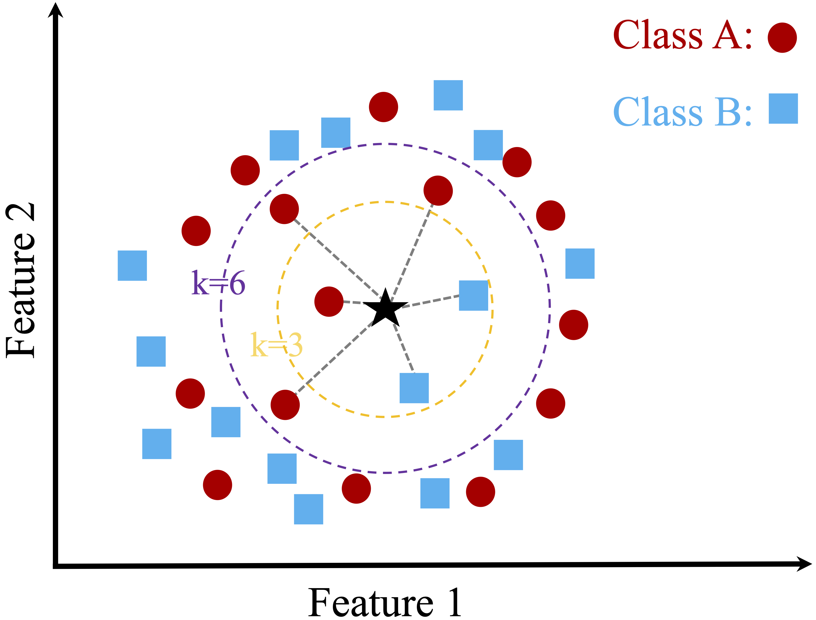
Figure 7.1: A two-dimensional toy dataset with two classes (Class A and Class B) and a new data point (dark star), illustrating the k-Nearest Neighbors algorithm with k = 3 and k = 6.

These examples illustrate how the choice of $k$ affects classification. A smaller $k$ (e.g., 3) makes predictions highly sensitive to local patterns, capturing finer details but also increasing the risk of misclassification due to noise. In contrast, a larger $k$ (e.g., 6) smooths predictions by incorporating more neighbors, reducing sensitivity to individual data points but potentially overlooking localized structures in the data. Selecting an appropriate $k$ ensures that kNN generalizes well without becoming overly complex or overly simplistic.

Strengths and Limitations of kNN

The kNN algorithm is widely used due to its simplicity and intuitive nature, making it an excellent starting point for classification problems. By relying only on distance metrics and majority voting, it avoids the complexity of training explicit models. However, this simplicity comes with trade-offs, particularly in handling large datasets and noisy features.

One of kNN’s key strengths is its ease of implementation and interpretability. Since it does not require model training, it can be applied directly to datasets with minimal preprocessing. It performs well on small datasets where patterns are well-defined and feature relationships are strong. However, kNN is highly sensitive to irrelevant or noisy features, as distance calculations may become less meaningful when unnecessary attributes are included. Additionally, it can be computationally expensive for large datasets, since it must calculate distances for every training point during prediction. The choice of $k$ also plays a crucial role—too small a $k$ makes the algorithm overly sensitive to noise, while too large a $k$ may oversimplify patterns, leading to reduced accuracy.

kNN in Action: A Toy Example for Drug Classification

To further illustrate kNN, consider a real-world scenario involving drug prescription classification. A dataset of 200 patients includes their age, sodium-to-potassium (Na/K) ratio, and the drug type they were prescribed. This dataset is synthetically generated to reflect a real-world scenario. For details on how this dataset was generated, refer to Section 1.16. Figure 7.2 visualizes this dataset, where different drug types are represented by:

• Red circles for Drug A,
  
• Green triangles for Drug B, and
  
• Blue squares for Drug C.

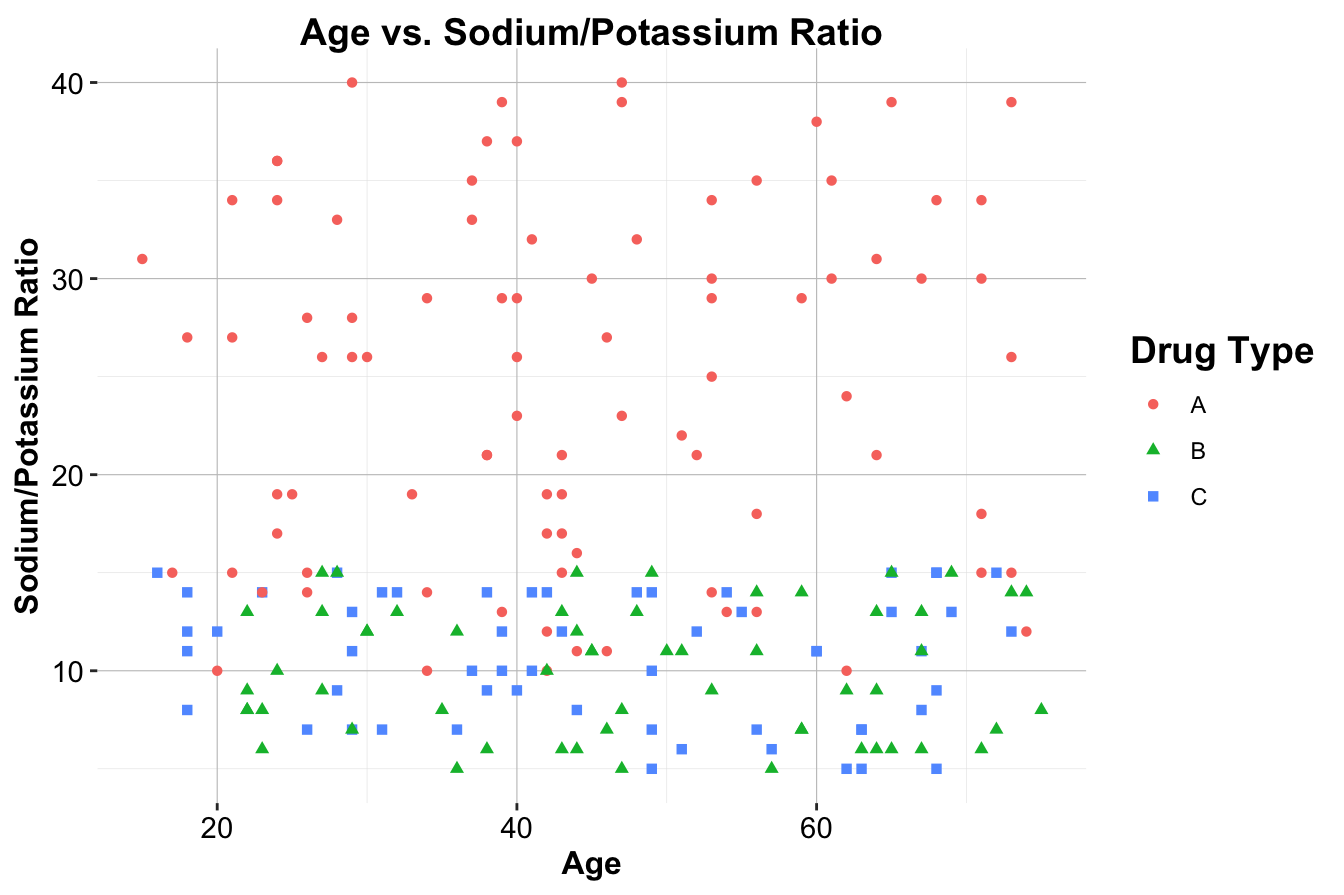
Figure 7.2: Scatter plot of Age vs. Sodium/Potassium Ratio for 200 patients, with drug type indicated by color and shape.

Suppose three new patients arrive at the clinic, and we need to determine which drug is most suitable for them based on their age and sodium-to-potassium ratio. Their details are as follows:

1. Patient 1: 40 years old with a Na/K ratio of 30.5.
   
2. Patient 2: 28 years old with a Na/K ratio of 9.6.
   
3. Patient 3: 61 years old with a Na/K ratio of 10.5.

These patients are represented as orange circles in Figure 7.3. Using kNN, we will classify the drug type for each patient.

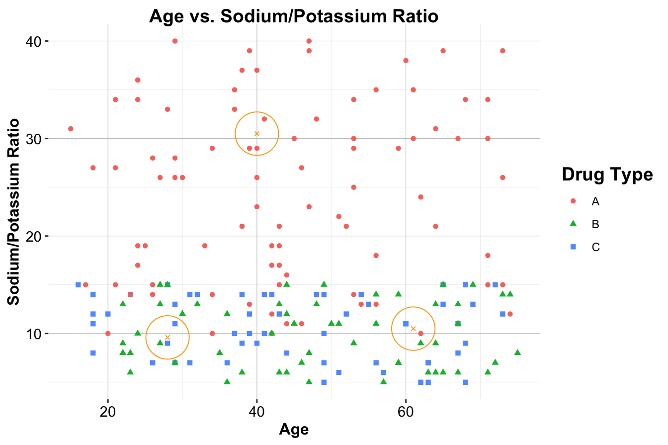
Figure 7.3: Scatter plot of Age vs. Sodium/Potassium Ratio for 200 patients, with drug type indicated by color and shape. The three new patients are represented by large orange circles.

For Patient 1, who is located deep within a cluster of red-circle points (Drug A), the classification is straightforward: Drug A. All the nearest neighbors belong to Drug A, making it an easy decision.

For Patient 2, the situation is more nuanced. If $k=1$, the nearest neighbor is a blue square, resulting in the classification Drug C. When $k=2$, there is a tie between Drug B and Drug C, leading to no clear majority. With $k=3$, two out of the three nearest neighbors are blue squares, so the classification remains Drug C.

For Patient 3, classification becomes even more ambiguous. With $k=1$, the closest neighbor is a blue square, classifying the patient as Drug C. However, for $k=2$ or $k=3$, the nearest neighbors belong to multiple classes, creating uncertainty in classification.

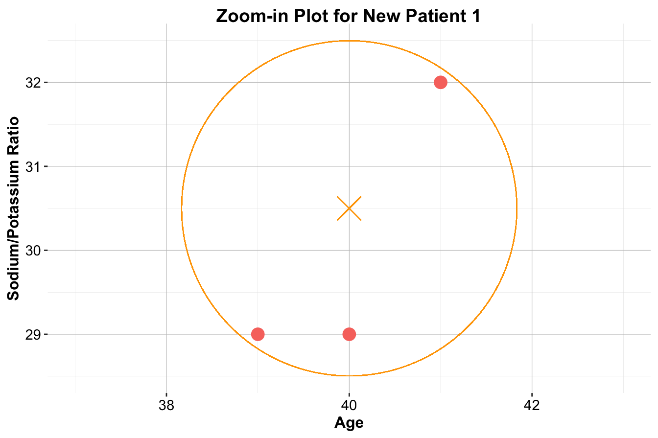
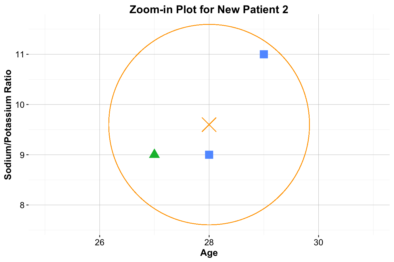
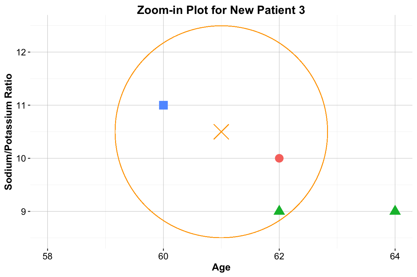
Figure 7.4: Zoom-in plots for the three new patients and their nearest neighbors. The left plot is for Patient 1, the middle plot is for Patient 2, and the right plot is for Patient 3.

These examples highlight several key aspects of kNN. The choice of $k$ significantly influences classification—small values of $k$ make the algorithm highly sensitive to local patterns, while larger values introduce smoothing by considering broader neighborhoods. Additionally, the selection of distance metrics, such as Euclidean distance, affects how neighbors are determined. Finally, proper feature scaling ensures that all variables contribute fairly to distance calculations, preventing dominance by features with larger numeric ranges.

This example demonstrates how kNN assigns labels based on proximity, reinforcing the importance of thoughtful parameter selection and preprocessing techniques. Before applying kNN to real-world datasets, it is essential to understand how similarity is measured—this leads to the next discussion on distance metrics.

7.3 Distance Metrics

In the kNN algorithm, the classification of a new data point is determined by identifying the most similar records from the training dataset. But how do we define and measure similarity? While similarity might seem intuitive, applying it in machine learning requires precise distance metrics. These metrics quantify the “closeness” between two data points in a multidimensional space, directly influencing how neighbors are selected for classification.

Imagine you’re shopping online and looking for recommendations. You’re a 50-year-old married female—who’s more similar to you: a 40-year-old single female or a 30-year-old married male? The answer depends on how we measure the distance between you and each person. In kNN, this distance is computed using numerical features such as age and categorical features such as marital status. The smaller the distance, the more “similar” two individuals are, and the more influence they have in determining predictions. Since kNN assumes that closer points (lower distance) belong to the same class, choosing the right distance metric is crucial for accurate classification.

Euclidean Distance

The most widely used distance metric in kNN is Euclidean distance, which measures the straight-line distance between two points. Think of it as the “as-the-crow-flies” distance, similar to the shortest path between two locations on a map. This metric is intuitive and aligns with how we often perceive distance in the real world.

Mathematically, the Euclidean distance between two points, $x$ and $y$, in $n$-dimensional space is given by:

$$\text{dist}(x,y)=\sqrt{(x_1-y_1{)}^2+(x_2-y_2{)}^2+\dots +(x_n-y_n{)}^2},$$

where $x=(x_1,x_2,\dots ,x_n)$ and $y=(y_1,y_2,\dots ,y_n)$ represent the feature vectors of the two points. The differences between corresponding features ($x_i-y_i$) are squared, summed, and then square-rooted to calculate the distance.

Example 7.1 Let’s calculate the Euclidean distance between two patients based on their age and sodium-to-potassium (Na/K) ratio:

• Patient 1: $x=(40,30.5)$
  
• Patient 2: $y=(28,9.6)$

Using the formula:
$$\text{dist}(x,y)=\sqrt{(40-28{)}^2+(30.5-9.6{)}^2}=\sqrt{(12{)}^2+(20.9{)}^2}=24.11$$

This result quantifies the dissimilarity between the two patients. In kNN, this distance helps determine how similar Patient 1 is to Patient 2 and whether they should be classified into the same drug class.

Choosing the Right Distance Metric

While Euclidean distance is widely used in kNN, it is not always the best choice. Other distance metrics can be more suitable depending on the dataset’s characteristics:

• Manhattan Distance: Measures distance by summing the absolute differences between coordinates. This is useful when movement is restricted to grid-like paths, such as city blocks.
• Hamming Distance: Used for categorical variables, where the distance is the number of positions at which two feature vectors differ.
• Cosine Similarity: Measures the angle between two vectors rather than their absolute distance. This is useful in high-dimensional spaces, such as text classification.

The choice of distance metric depends on the data type and problem domain. If your dataset contains categorical or high-dimensional features, exploring alternative metrics—such as Manhattan or Cosine Similarity—might be necessary. For further details, refer to the dist() function in R.

7.4 How to Choose an Optimal $k$

How many opinions do you seek before making an important decision? Too few might lead to a biased perspective, while too many might dilute the relevance of the advice. Similarly, in the k-Nearest Neighbors (kNN) algorithm, the choice of $k$—the number of neighbors considered for classification—directly impacts the model’s performance. But how do we determine the right $k$?

There is no universally “correct” value for $k$. The optimal choice depends on the specific dataset and classification problem, requiring careful consideration of the trade-offs involved.

Balancing Overfitting and Underfitting

When $k$ is too small, such as $k=1$, the algorithm becomes highly sensitive to individual training points. Each new observation is classified based on its single closest neighbor, making the model highly reactive to noise and outliers. This can lead to overfitting, where the model memorizes the training data but fails to generalize to unseen data. For example, a small cluster of mislabeled data points could disproportionately influence predictions, reducing the model’s reliability.

Conversely, as $k$ increases, the algorithm incorporates more neighbors into the classification decision. Larger $k$ values smooth the decision boundary, reducing the impact of noise and outliers. However, if $k$ is too large, the model may oversimplify, averaging out meaningful patterns in the data. When $k$ is comparable to the size of the training set, the majority class dominates predictions, leading to underfitting, where the model fails to capture important distinctions.

Choosing an appropriate $k$ requires balancing these extremes. Smaller values of $k$ capture fine-grained local structures but risk overfitting, while larger values provide more stability at the expense of detail.

Choosing $k$ Through Validation

Since the optimal $k$ depends on the dataset, a common approach is to evaluate multiple values of $k$ using a validation set or cross-validation. Performance metrics such as accuracy, precision, recall, and F1-score help identify the best $k$ for a given problem.

To illustrate, we use the churn dataset and evaluate the accuracy of the kNN algorithm across different $k$ values (ranging from 1 to 30). Figure 7.5 shows how accuracy fluctuates as $k$ increases. The plot is generated using the kNN.plot() function from the liver package in R.

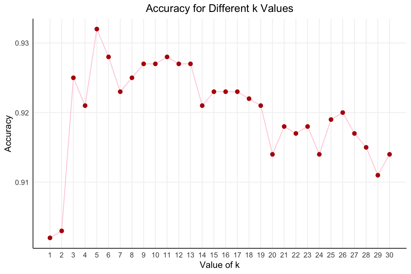
Figure 7.5: Accuracy of the k-Nearest Neighbors algorithm for different values of k in the range from 1 to 30.

From the plot, we observe that kNN accuracy fluctuates as $k$ increases. The highest accuracy is achieved when $k=5$, where the algorithm balances sensitivity to local patterns with robustness to noise. At this value, kNN delivers an accuracy of 0.932 and an error rate of 0.068.

Choosing the optimal $k$ is as much an art as it is a science. While there’s no universal rule for selecting $k$, experimentation and validation are key. Start with a range of plausible $k$ values, test the model’s performance, and select the one that provides the best results based on your chosen metric.

Keep in mind that the optimal $k$ may vary across datasets. Whenever applying kNN to a new problem, repeating this process ensures the model remains both accurate and generalizable. By carefully tuning $k$, we strike the right balance between overfitting and underfitting, improving the model’s predictive power.

7.5 Preparing Data for kNN

The effectiveness of the kNN algorithm relies heavily on how the dataset is prepared. Since kNN uses distance metrics to evaluate similarity between data points, proper preprocessing is crucial to ensure accurate and meaningful results. Two essential steps in this process are feature scaling and one-hot encoding, which enable the algorithm to handle numerical and categorical features effectively. These steps are part of the Preparing Data for Modeling stage in the Data Science Workflow (Figure 2.3).

7.5.1 Feature Scaling

In most datasets, numerical features often have vastly different ranges. For instance, age may range from 20 to 70, while income could range from 20,000 to 150,000. Without proper scaling, features with larger ranges, such as income, will dominate distance calculations, leading to biased predictions. To address this, all numerical features must be transformed to comparable scales. See Section 3.5 for more details on scaling methods.

A widely used method is min-max scaling, which transforms each feature to a specified range, typically $[0,1]$, using the formula: $$x_{\text{scaled}}=\frac{x-min\left(x\right)}{max\left(x\right)-min\left(x\right)},$$ where $x$ represents the original feature value, and $min\left(x\right)$ and $max\left(x\right)$ are the minimum and maximum values of the feature, respectively. This formula rescales each feature to a $[0,1]$ range, ensuring that no single feature dominates the distance calculation.

Another common method is z-score standardization, which rescales features so that they have a mean of 0 and a standard deviation of 1: $$x_{\text{scaled}}=\frac{x-\text{mean}\left(x\right)}{\text{sd}\left(x\right)}$$ This method is particularly useful when features contain outliers or follow different distributions. Unlike min-max scaling, z-score standardization does not constrain values within a fixed range but ensures that they follow a standard normal distribution, making it more robust to extreme values.

Choosing the Right Scaling Method:
Min-max scaling is preferable when feature values are bounded within a known range, such as pixel values in images or percentages. This ensures that all features contribute equally to the distance metric while maintaining their relative proportions. On the other hand, z-score standardization is more suitable when data contains extreme values or follows different distributions across features. It transforms values into a standard normal distribution, making it particularly effective for datasets with outliers or varying units of measurement.

Avoiding Data Leakage: Scaling must always be performed after partitioning the dataset into training and test sets. The scaling parameters, such as the minimum and maximum for min-max scaling or the mean and standard deviation for z-score standardization, should be computed from the training set only and then applied consistently to both the training and test sets. Performing scaling before partitioning can introduce data leakage, where information from the test set inadvertently influences the training process. This can lead to misleadingly high accuracy during evaluation, as the model indirectly gains access to test data before making predictions.

7.5.2 Scaling Training and Test Data the Same Way

To illustrate the importance of consistent scaling, consider the patient drug classification problem, which involves two features: age and sodium/potassium (Na/K) ratio. Figure 7.3 shows a dataset of 200 patients as the training set, with three additional patients in the test set. Using the minmax() function from the liver package, we demonstrate both correct and incorrect ways to scale the data:

# Load the liver package
library(liver)

# A proper way to scale the data
train_scaled = minmax(train_data, col = c("Age", "Ratio"))

test_scaled = minmax(test_data, col = c("Age", "Ratio"), min = c(min(train_data$Age), min(train_data$Ratio)), max = c(max(train_data$Age), max(train_data$Ratio)))

# An incorrect way to scale the data
train_scaled_wrongly = minmax(train_data, col = c("Age", "Ratio"))
test_scaled_wrongly  = minmax(test_data , col = c("Age", "Ratio"))

The difference is illustrated in Figure 7.6. The middle panel shows the results of proper scaling, where the test set is scaled using the same parameters derived from the training set. This ensures consistency in distance calculations across both datasets. In contrast, the right panel shows improper scaling, where the test set is scaled independently. This leads to distorted relationships between the training and test data, which can cause unreliable predictions.

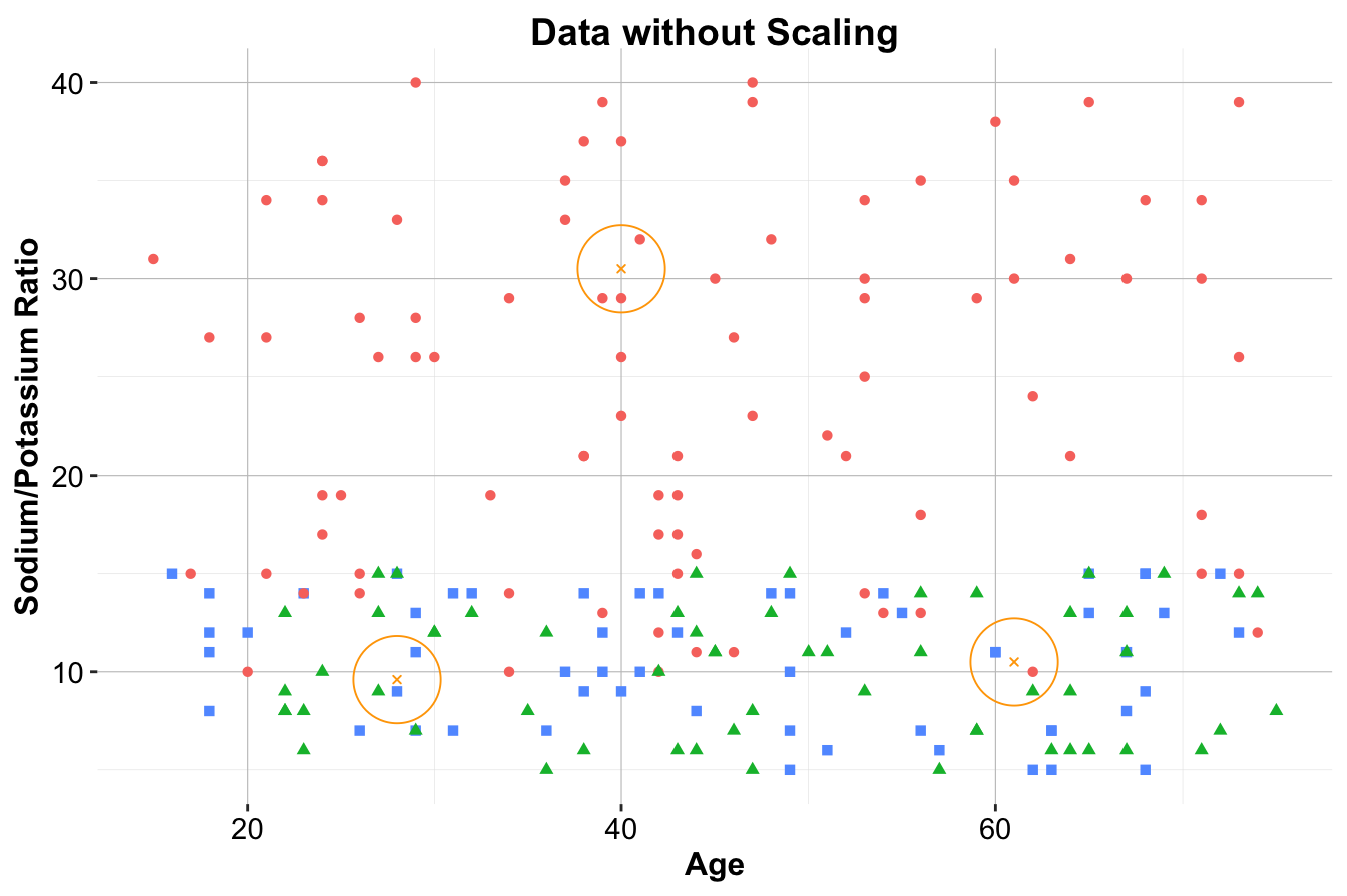
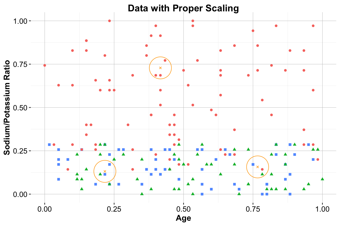
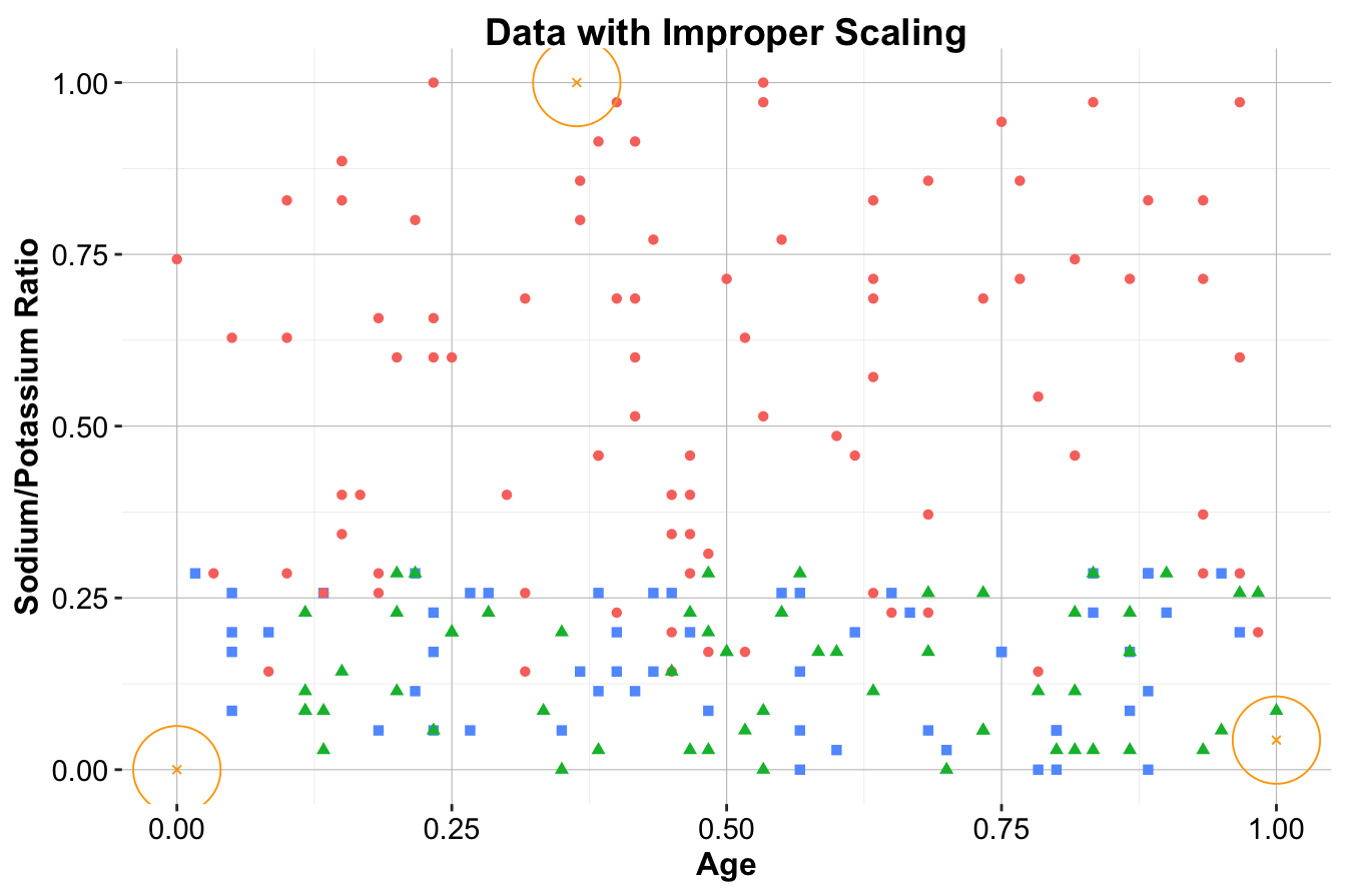
Figure 7.6: Visualization illustrating the difference between proper scaling and improper scaling. The left panel shows the original data without scaling. The middle panel shows the results of proper scaling. The right panel shows the results of improper scaling.

Key Insight: Proper scaling ensures that distance metrics remain valid, while improper scaling creates inconsistencies that undermine the kNN algorithm’s performance. Scaling parameters should always be derived from the training set and applied consistently to the test set. Neglecting this principle introduces data leakage, which distorts model evaluation and leads to overly optimistic performance estimates.

7.5.3 One-Hot Encoding

Categorical features, such as marital status or subscription type, cannot be directly used in distance calculations because distance metrics like Euclidean distance only work with numerical data. To overcome this, we use one-hot encoding, which converts categorical variables into binary (dummy) variables.

For example, the categorical variable voice.plan, with levels yes and no, can be encoded as:

$$\text{voice.plan-yes}=\{\begin{array}{c}1\text{if voice plan = yes}\\ 0\text{if voice plan = no}\end{array}$$

For categorical variables with more than two categories, one-hot encoding creates multiple binary columns—one for each category except one, to avoid redundancy. This approach ensures that the categorical variable is fully represented without introducing unnecessary correlations.

The liver package in R provides the one.hot() function to perform one-hot encoding automatically. It identifies categorical variables and encodes them into binary columns, leaving numerical features unchanged. Applying one-hot encoding to the marital variable in the bank dataset, for instance, adds binary columns for the encoded categories:

data(bank)

# To perform one-hot encoding on the "marital" variable
bank_encoded <- one.hot(bank, cols = c("marital"), dropCols = FALSE)

str(bank_encoded)
   'data.frame':    4521 obs. of  20 variables:
    $ age             : int  30 33 35 30 59 35 36 39 41 43 ...
    $ job             : Factor w/ 12 levels "admin.","blue-collar",..: 11 8 5 5 2 5 7 10 3 8 ...
    $ marital         : Factor w/ 3 levels "divorced","married",..: 2 2 3 2 2 3 2 2 2 2 ...
    $ marital_divorced: int  0 0 0 0 0 0 0 0 0 0 ...
    $ marital_married : int  1 1 0 1 1 0 1 1 1 1 ...
    $ marital_single  : int  0 0 1 0 0 1 0 0 0 0 ...
    $ education       : Factor w/ 4 levels "primary","secondary",..: 1 2 3 3 2 3 3 2 3 1 ...
    $ default         : Factor w/ 2 levels "no","yes": 1 1 1 1 1 1 1 1 1 1 ...
    $ balance         : int  1787 4789 1350 1476 0 747 307 147 221 -88 ...
    $ housing         : Factor w/ 2 levels "no","yes": 1 2 2 2 2 1 2 2 2 2 ...
    $ loan            : Factor w/ 2 levels "no","yes": 1 2 1 2 1 1 1 1 1 2 ...
    $ contact         : Factor w/ 3 levels "cellular","telephone",..: 1 1 1 3 3 1 1 1 3 1 ...
    $ day             : int  19 11 16 3 5 23 14 6 14 17 ...
    $ month           : Factor w/ 12 levels "apr","aug","dec",..: 11 9 1 7 9 4 9 9 9 1 ...
    $ duration        : int  79 220 185 199 226 141 341 151 57 313 ...
    $ campaign        : int  1 1 1 4 1 2 1 2 2 1 ...
    $ pdays           : int  -1 339 330 -1 -1 176 330 -1 -1 147 ...
    $ previous        : int  0 4 1 0 0 3 2 0 0 2 ...
    $ poutcome        : Factor w/ 4 levels "failure","other",..: 4 1 1 4 4 1 2 4 4 1 ...
    $ deposit         : Factor w/ 2 levels "no","yes": 1 1 1 1 1 1 1 1 1 1 ...

Setting dropCols = FALSE retains the original categorical column in the dataset, which may be useful for reference or debugging. However, in most cases, it is recommended to remove the original column after encoding to avoid redundancy.

Note: One-hot encoding is unnecessary for ordinal features, where the categories have a natural order (e.g., low, medium, high). Ordinal variables should instead be assigned numerical values that preserve their order (e.g., low = 1, medium = 2, high = 3), enabling the kNN algorithm to treat them as numerical features. For instance, if education.level has values {low, medium, high}, one-hot encoding would lose the natural progression between these categories. Instead, assigning numerical values (low = 1, medium = 2, high = 3) allows the algorithm to recognize the ordinal nature of the feature, preserving its relationship in distance calculations.

7.6 Applying kNN Algorithm in Practice

Applying the kNN algorithm involves several key steps, from preparing the data to training the model, making predictions, and evaluating its performance. In this section, we demonstrate the entire workflow using the churn dataset from the liver package in R. The target variable, churn, indicates whether a customer has churned (yes) or not (no), while the predictors include customer characteristics such as account length, international plan status, and call details. For details on exploratory data analysis, problem understanding, and data preparation for this dataset, refer to Section 4.3.

str(churn)
   'data.frame':    5000 obs. of  20 variables:
    $ state         : Factor w/ 51 levels "AK","AL","AR",..: 17 36 32 36 37 2 20 25 19 50 ...
    $ area.code     : Factor w/ 3 levels "area_code_408",..: 2 2 2 1 2 3 3 2 1 2 ...
    $ account.length: int  128 107 137 84 75 118 121 147 117 141 ...
    $ voice.plan    : Factor w/ 2 levels "yes","no": 1 1 2 2 2 2 1 2 2 1 ...
    $ voice.messages: int  25 26 0 0 0 0 24 0 0 37 ...
    $ intl.plan     : Factor w/ 2 levels "yes","no": 2 2 2 1 1 1 2 1 2 1 ...
    $ intl.mins     : num  10 13.7 12.2 6.6 10.1 6.3 7.5 7.1 8.7 11.2 ...
    $ intl.calls    : int  3 3 5 7 3 6 7 6 4 5 ...
    $ intl.charge   : num  2.7 3.7 3.29 1.78 2.73 1.7 2.03 1.92 2.35 3.02 ...
    $ day.mins      : num  265 162 243 299 167 ...
    $ day.calls     : int  110 123 114 71 113 98 88 79 97 84 ...
    $ day.charge    : num  45.1 27.5 41.4 50.9 28.3 ...
    $ eve.mins      : num  197.4 195.5 121.2 61.9 148.3 ...
    $ eve.calls     : int  99 103 110 88 122 101 108 94 80 111 ...
    $ eve.charge    : num  16.78 16.62 10.3 5.26 12.61 ...
    $ night.mins    : num  245 254 163 197 187 ...
    $ night.calls   : int  91 103 104 89 121 118 118 96 90 97 ...
    $ night.charge  : num  11.01 11.45 7.32 8.86 8.41 ...
    $ customer.calls: int  1 1 0 2 3 0 3 0 1 0 ...
    $ churn         : Factor w/ 2 levels "yes","no": 2 2 2 2 2 2 2 2 2 2 ...

The dataset is a data.frame in R with 5000 observations and 19 predictor variables. The target variable, churn, indicates whether a customer has churned (yes) or not (no).

Based on insights gained in Section 4.3, we select the following features for building the kNN model:

account.length, voice.plan, voice.messages, intl.plan, intl.mins, day.mins, eve.mins, night.mins, and customer.calls.

The next steps involve preparing the data through feature scaling and one-hot encoding, followed by selecting an optimal $k$, training the kNN model, and evaluating its performance.

7.6.1 Step 1: Preparing the Data

The first step in applying kNN is to partition the dataset into training and test sets, followed by preprocessing tasks like feature scaling and one-hot encoding. Since the dataset is already cleaned and free of missing values, we can proceed directly with partitioning before applying these transformations.

We split the dataset into an 80% training set and a 20% test set using the partition() function from the liver package:

set.seed(43)

data_sets = partition(data = churn, ratio = c(0.8, 0.2))

train_set = data_sets$part1
test_set  = data_sets$part2

test_labels = test_set$churn

The partition() function randomly splits the dataset while maintaining the class distribution of the target variable, ensuring a representative training and test set. As we validated the partition in Section 6.4, we can now proceed with feature scaling and one-hot encoding to ensure compatibility with the kNN algorithm.

One-Hot Encoding

Since kNN relies on distance calculations, categorical variables like voice.plan and intl.plan must be converted into numerical representations. One-hot encoding achieves this by creating binary (dummy) variables for each category. We apply the one.hot() function from the liver package to transform categorical features into a numerical format suitable for kNN:

categorical_vars = c("voice.plan", "intl.plan")

train_onehot = one.hot(train_set, cols = categorical_vars)
test_onehot  = one.hot(test_set,  cols = categorical_vars)

str(test_onehot)
   'data.frame':    1000 obs. of  22 variables:
    $ state         : Factor w/ 51 levels "AK","AL","AR",..: 2 50 14 46 10 4 25 15 11 32 ...
    $ area.code     : Factor w/ 3 levels "area_code_408",..: 3 2 1 3 2 2 2 2 2 1 ...
    $ account.length: int  118 141 85 76 147 130 20 142 72 149 ...
    $ voice.plan_yes: int  0 1 1 1 0 0 0 0 1 0 ...
    $ voice.plan_no : int  1 0 0 0 1 1 1 1 0 1 ...
    $ voice.messages: int  0 37 27 33 0 0 0 0 37 0 ...
    $ intl.plan_yes : int  1 1 0 0 0 0 0 0 0 0 ...
    $ intl.plan_no  : int  0 0 1 1 1 1 1 1 1 1 ...
    $ intl.mins     : num  6.3 11.2 13.8 10 10.6 9.5 6.3 14.2 14.7 11.1 ...
    $ intl.calls    : int  6 5 4 5 4 19 6 6 6 9 ...
    $ intl.charge   : num  1.7 3.02 3.73 2.7 2.86 2.57 1.7 3.83 3.97 3 ...
    $ day.mins      : num  223 259 196 190 155 ...
    $ day.calls     : int  98 84 139 66 117 112 109 95 80 94 ...
    $ day.charge    : num  38 44 33.4 32.2 26.4 ...
    $ eve.mins      : num  221 222 281 213 240 ...
    $ eve.calls     : int  101 111 90 65 93 99 84 63 102 92 ...
    $ eve.charge    : num  18.8 18.9 23.9 18.1 20.4 ...
    $ night.mins    : num  203.9 326.4 89.3 165.7 208.8 ...
    $ night.calls   : int  118 97 75 108 133 78 102 148 71 108 ...
    $ night.charge  : num  9.18 14.69 4.02 7.46 9.4 ...
    $ customer.calls: int  0 0 1 1 0 0 0 2 3 1 ...
    $ churn         : Factor w/ 2 levels "yes","no": 2 2 2 2 2 2 2 2 2 2 ...

For binary categorical variables, one-hot encoding produces two columns (e.g., voice.plan_yes and voice.plan_no). Since one variable is always the complement of the other, we retain only one (e.g., voice.plan_yes) to avoid redundancy.

Feature Scaling

Since kNN calculates distances between data points, features with larger numerical ranges can disproportionately influence the results. Scaling ensures that all features contribute equally to distance calculations, preventing dominance by high-magnitude features.

To standardize the numerical variables, we apply min-max scaling using the minmax() function from the liver package. Scaling parameters (minimum and maximum values) must be computed from the training set and then applied consistently to both the training and test sets. This prevents data leakage, which occurs when test data influences the training process, leading to misleadingly high performance estimates.

numeric_vars = c("account.length", "voice.messages", "intl.mins", 
                 "intl.calls", "day.mins", "day.calls", "eve.mins", 
                 "eve.calls", "night.mins", "night.calls", 
                 "customer.calls")

min_train = sapply(train_set[, numeric_vars], min)
max_train = sapply(train_set[, numeric_vars], max)

train_scaled = minmax(train_onehot, col = numeric_vars, min = min_train, max = max_train)
test_scaled  = minmax(test_onehot,  col = numeric_vars, min = min_train, max = max_train)

The minmax() function normalizes the numerical features to the range $[0,1]$, ensuring they have comparable scales while preserving relative differences. This transformation prevents any single feature from dominating the kNN distance calculations, leading to more balanced and accurate predictions.

7.6.2 Step 2: Choosing an Optimal $k$

The selection of $k$ plays a crucial role in balancing local pattern recognition and generalization to unseen data. A small $k$ may lead to overfitting, making the model highly sensitive to noise, while a large $k$ can result in oversmoothing, causing the model to overlook important details. To find an optimal $k$, we evaluate the model’s accuracy across different values of $k$ and select the one that yields the best performance.

A practical way to achieve this is by plotting model accuracy against different values of $k$. The kNN.plot() function from the liver package automates this process, providing a clear visualization of the relationship between $k$ and accuracy:

formula = churn ~ account.length + voice.plan_yes + voice.messages + 
                  intl.plan_yes + intl.mins + intl.calls + 
                  day.mins + day.calls + eve.mins + eve.calls + 
                  night.mins + night.calls + customer.calls

kNN.plot(formula = formula, train = train_scaled, test = test_scaled, 
         k.max = 30, set.seed = 43)
   Setting levels: reference = "yes", case = "no"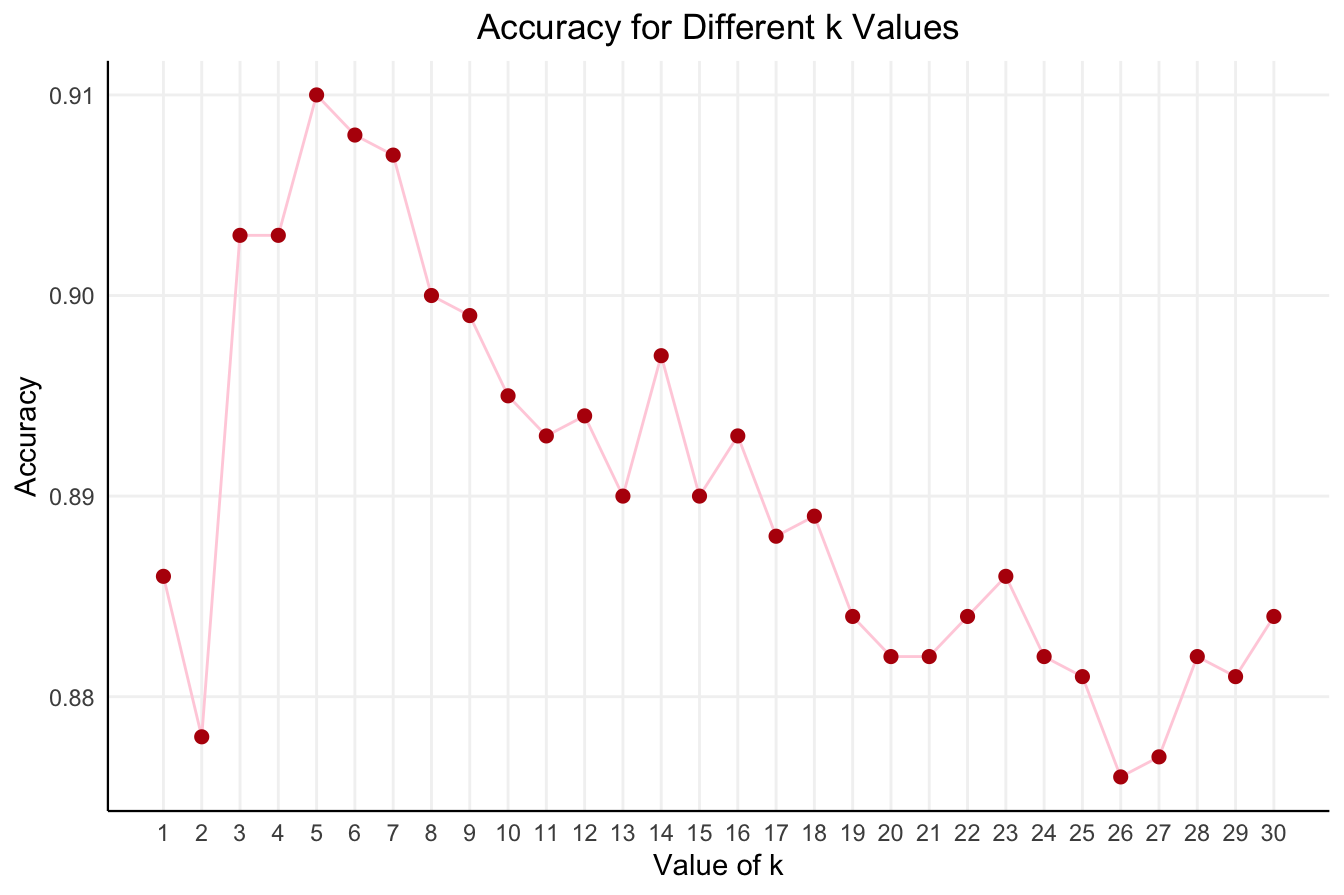

The resulting plot helps identify the optimal $k$, balancing model complexity and generalization. From the visualization, we observe that the highest accuracy is achieved when $k=5$, suggesting that this value effectively captures meaningful patterns while minimizing sensitivity to outliers.

7.6.3 Step 3: Training the Model and Making Predictions

With $k=5$ identified as the optimal value, we are now ready to classify test records using the k-NN algorithm. Unlike many machine learning methods, k-NN is a lazy learner, meaning it does not build an explicit model during training. Instead, it simply stores the training data in a structured format and performs classification only when a new observation needs to be classified.

Several R packages provide implementations of the k-NN algorithm, including class and liver. The class package offers basic k-NN functionality, while the liver package provides an enhanced kNN() function that supports a formula-based interface and built-in normalization.

To apply the k-NN algorithm, we use the kNN() function from the liver package:

kNN_predict = kNN(formula = formula, train = train_scaled, test = test_scaled, k = 5)

In this function:

• formula specifies the relationship between the target variable and predictors.
  
• train contains the scaled training data.
  
• test contains the scaled test data.
  
• k determines the number of nearest neighbors to consider, set here to $k=5$ based on the selection in the previous step.

The kNN() function classifies test observations by computing distances between each test record and all training data points. It then selects the five closest neighbors based on the chosen distance metric and assigns the most frequent class among them as the predicted label. Since test data is independent of training data, these predictions provide an unbiased estimate of the model’s ability to generalize to new observations.

7.6.4 Step 4: Evaluating the Model

Evaluating model performance is crucial to ensure that the kNN algorithm generalizes well to unseen data and makes reliable predictions. A confusion matrix provides a summary of correct and incorrect predictions by comparing the predicted labels to the actual labels in the test set. We compute it using the conf.mat() function from the liver package:

conf.mat(kNN_predict, test_labels, reference = "yes")
          Actual
   Predict yes  no
       yes  54   7
       no   83 856

From the confusion matrix, we see that the model correctly classified 910 instances, while 90 instances were misclassified. This summary helps assess model performance and identify areas for improvement.

Final Remarks

This step-by-step implementation of kNN highlighted the crucial role of data preprocessing, parameter tuning, and model evaluation in achieving reliable predictions. Key factors such as the choice of $k$, feature scaling, and encoding categorical data significantly influence the accuracy and generalization of kNN models.

While the confusion matrix provides an initial assessment of model performance, additional evaluation metrics such as accuracy, precision, recall, and F1-score offer deeper insights. These aspects will be explored in detail in the next chapter (Chapter 8).

7.7 Key Takeaways from kNN

In this chapter, we explored the k-Nearest Neighbors (kNN) algorithm, a simple yet effective method for solving classification problems. We began by revisiting the concept of classification and its real-world applications, highlighting the difference between binary and multi-class problems. We then examined the mechanics of kNN, emphasizing its reliance on distance metrics to identify the most similar data points. Essential preprocessing steps, such as feature scaling and one-hot encoding, were discussed to ensure accurate and meaningful distance calculations. We also covered the importance of selecting an optimal $k$ value and demonstrated the implementation of kNN using the liver package in R with the churn dataset. Through practical examples, we reinforced the significance of proper data preparation and parameter tuning for building reliable classification models.

The simplicity and interpretability of kNN make it an excellent starting point for understanding classification and exploring dataset structures. However, the algorithm has notable limitations, including sensitivity to noise, computational inefficiency with large datasets, and the necessity for proper scaling and feature selection. These challenges make kNN less practical for large-scale applications, but it remains a valuable tool for small to medium-sized datasets and serves as a benchmark for evaluating more advanced algorithms.

While kNN is intuitive and easy to implement, its prediction speed and scalability constraints often limit its use in modern, large-scale datasets. Nonetheless, it is a useful baseline method and a stepping stone to more sophisticated techniques. In the upcoming chapters, we will explore advanced classification algorithms, such as Decision Trees, Random Forests, and Logistic Regression, which address the limitations of kNN and provide enhanced performance and scalability for a wide range of applications.

7.8 Exercises

Conceptual Questions

1. Explain the fundamental difference between classification and regression. Provide an example of each.
   
2. What are the key steps in applying the kNN algorithm?
   
3. Why is the choice of $k$ important in kNN, and what happens when $k$ is too small or too large?
   
4. Describe the role of distance metrics in kNN classification. Why is Euclidean distance commonly used?
   
5. What are the limitations of kNN compared to other classification algorithms?
   
6. How does feature scaling impact the performance of kNN? Why is it necessary?
   
7. Describe how one-hot encoding is used in kNN. Why is it necessary for categorical variables?
   
8. How does kNN handle missing values? What strategies can be used to deal with missing data?
   
9. Explain the difference between lazy learning (such as kNN) and eager learning (such as decision trees or logistic regression).
   
10. Why is kNN considered a non-parametric algorithm? What advantages and disadvantages does this bring?

Hands-On Practice: Applying kNN to the Bank Dataset

Here, we want to apply the concepts covered in this chapter using the bank dataset from the liver package. The bank dataset contains customer information, including demographics and financial details, and the target variable deposit indicates whether a customer subscribed to a term deposit. This dataset is well-suited for classification problems and provides an opportunity to practice kNN in real-world scenarios.

To begin, load the necessary package and dataset:

library(liver)

# Load the dataset
data(bank)

# View the structure of the dataset
str(bank)
   'data.frame':    4521 obs. of  17 variables:
    $ age      : int  30 33 35 30 59 35 36 39 41 43 ...
    $ job      : Factor w/ 12 levels "admin.","blue-collar",..: 11 8 5 5 2 5 7 10 3 8 ...
    $ marital  : Factor w/ 3 levels "divorced","married",..: 2 2 3 2 2 3 2 2 2 2 ...
    $ education: Factor w/ 4 levels "primary","secondary",..: 1 2 3 3 2 3 3 2 3 1 ...
    $ default  : Factor w/ 2 levels "no","yes": 1 1 1 1 1 1 1 1 1 1 ...
    $ balance  : int  1787 4789 1350 1476 0 747 307 147 221 -88 ...
    $ housing  : Factor w/ 2 levels "no","yes": 1 2 2 2 2 1 2 2 2 2 ...
    $ loan     : Factor w/ 2 levels "no","yes": 1 2 1 2 1 1 1 1 1 2 ...
    $ contact  : Factor w/ 3 levels "cellular","telephone",..: 1 1 1 3 3 1 1 1 3 1 ...
    $ day      : int  19 11 16 3 5 23 14 6 14 17 ...
    $ month    : Factor w/ 12 levels "apr","aug","dec",..: 11 9 1 7 9 4 9 9 9 1 ...
    $ duration : int  79 220 185 199 226 141 341 151 57 313 ...
    $ campaign : int  1 1 1 4 1 2 1 2 2 1 ...
    $ pdays    : int  -1 339 330 -1 -1 176 330 -1 -1 147 ...
    $ previous : int  0 4 1 0 0 3 2 0 0 2 ...
    $ poutcome : Factor w/ 4 levels "failure","other",..: 4 1 1 4 4 1 2 4 4 1 ...
    $ deposit  : Factor w/ 2 levels "no","yes": 1 1 1 1 1 1 1 1 1 1 ...

Data Exploration and Preparation

11. Load the bank dataset and display its structure. Identify the target variable and the predictor variables.
    
12. Count the number of instances where a customer subscribed to a term deposit (deposit = “yes”) versus those who did not (deposit = “no”). What does this tell you about the dataset?
    
13. Identify nominal variables in the dataset. Convert them into numerical features using one-hot encoding with the one.hot() function.
    
14. Partition the dataset into 80% training and 20% testing sets using the partition() function. Ensure the target variable remains proportionally distributed in both sets.
    
15. Validate the partitioning by comparing the class distribution of the target variable in the training and test sets.
    
16. Apply min-max scaling to numerical variables in both training and test sets. Ensure that the scaling parameters are derived from the training set only.

Choosing the Optimal $k$

17. Use the kNN.plot() function to determine the optimal $k$ value for classifying deposit in the bank dataset.
    
18. What is the best $k$ value based on accuracy? How does accuracy change as $k$ increases?
19. Interpret the meaning of the accuracy curve generated by kNN.plot(). What patterns do you observe?

Building and Evaluating the kNN Model

20. Train a kNN model using the optimal $k$ and make predictions on the test set.
    
21. Generate a confusion matrix for the kNN model predictions using the conf.mat() function. Interpret the results.
    
22. Calculate the accuracy of the kNN model. How well does it perform in predicting deposit?
    
23. Besides accuracy, what other evaluation metrics (e.g., precision, recall, F1-score) would be useful for assessing kNN performance in the bank dataset? Compute and interpret these metrics.
    
24. Compare the performance of kNN with different values of $k$ (e.g., $k=1,5,15,25$). How does changing $k$ affect the classification results?
    
25. Train a kNN model using only a subset of features: age, balance, duration, and campaign. Compare its accuracy with the full-feature model. What does this tell you about feature selection?
    
26. Compare the accuracy of kNN when using min-max scaling versus z-score standardization. How does the choice of scaling method impact model performance?

Critical Thinking and Real-World Applications

27. Suppose you are building a fraud detection system for a bank. Would kNN be a suitable algorithm? What are its advantages and limitations in this context?
    
28. How would you handle imbalanced classes in the bank dataset? What strategies could improve classification performance?
    
29. In a high-dimensional dataset with hundreds of features, would kNN still be an effective approach? Why or why not?
    
30. Imagine you are working with a dataset where new data points arrive in real-time. What challenges would kNN face, and how could they be addressed?
    
31. If a financial institution wants to classify customers into different risk categories for loan approval, what preprocessing steps would be essential before applying kNN?
    
32. In a dataset where some features are irrelevant or redundant, how could you improve kNN’s performance? What feature selection methods would you use?
    
33. If computation time is a concern, what strategies could you apply to make kNN more efficient for large datasets?
    
34. Suppose kNN is performing poorly on the bank dataset. What possible reasons could explain this, and how would you troubleshoot the issue?