1 The Basics for R

Before you can analyze data, you need a way to communicate with your computer. That’s where programming languages like R and Python come in. Many data science teams use a mix of languages, but R is a great starting point because it is designed specifically for data analysis and statistical computing.

Why Choose R for Data Science?

R is widely used in statistics, data analysis, and visualization due to its rich ecosystem of libraries and tools tailored for data science. Unlike general-purpose programming languages, R was built for statistical analysis, allowing data scientists to perform everything from basic calculations to advanced machine learning with just a few lines of code.

While Python is another popular language for data science, R is particularly well-suited for: - Statistical Computing – R has built-in statistical functions and methods for hypothesis testing, regression modeling, and machine learning. - Data Visualization – Packages like ggplot2 provide powerful tools for creating high-quality plots and graphs with minimal effort. - Reproducible Research – R Markdown and Shiny make it easy to generate reports and interactive dashboards directly from R code. - Bioinformatics & Finance – Many researchers and analysts in these fields use R due to its robust statistical libraries and domain-specific packages.

Beyond its capabilities, R is:

Free & Open Source – Available to everyone, with a vibrant community of contributors.
Cross-Platform – Runs on Windows, macOS, and Linux.
Flexible & Powerful – Supports interactive data exploration, visualization, and machine learning.

While R is the language, RStudio is the tool that makes working with R easier. RStudio is an integrated development environment (IDE) that provides:

A console for running R commands,
A script editor with syntax highlighting and auto-completion,
Built-in tools for data visualization, debugging, and package management.

In this chapter, you will learn the fundamental skills needed to work with R, from installation to running your first commands. Let’s begin! 🚀

1.1 How to Install R

To get started with R, you first need to install it on your computer. Follow these steps:

Go to the CRAN website – The Comprehensive R Archive Network.
Select your operating system – Click the link for Windows, macOS, or Linux.
Download and install R – Follow the on-screen instructions to complete the installation.

Keeping R Up to Date

R receives a major update once a year, along with 2-3 minor updates annually. While updating R—especially major versions—requires reinstalling your packages, staying up to date ensures you:

✅ Access the latest features and improvements,
✅ Maintain compatibility with new packages,
✅ Benefit from security patches and performance enhancements.

Keeping R updated might feel like a hassle, but postponing updates can make the process more cumbersome later. It’s best to update regularly to ensure smooth performance and compatibility.

1.2 How to Install RStudio

RStudio is an open-source integrated development environment (IDE) that makes working with R easier, more interactive, and more efficient. It provides a user-friendly interface, an advanced script editor, and various tools for plotting, debugging, and workspace management—all of which significantly enhance the R programming experience.

Installing RStudio

Follow these steps to install RStudio:

Go to the RStudio website.
Download the latest version of RStudio Desktop (the free, open-source edition).
Run the installer and follow the on-screen instructions.
Launch RStudio, and you’re ready to start coding in R!

RStudio is updated several times a year, and it will notify you when a new version is available. Keeping RStudio up to date is recommended to take advantage of new features and performance improvements.

Exploring the RStudio Interface

When you open RStudio, you will see a window similar to Figure 1.1.

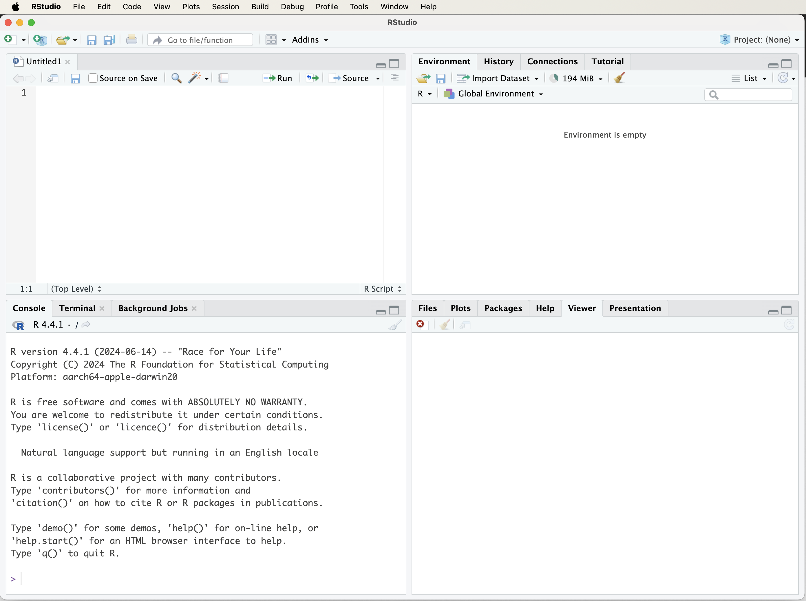
Figure 1.1: The RStudio window when you first launch the program.

If you see only three panels, add a fourth by selecting File > New File > R Script. This opens a script editor where you can write and save R code. Here’s a quick overview of RStudio’s panels:

Top-left: Script Editor – Write and save your R code.
Bottom-left: Console – Run R commands and see output.
Top-right: Environment & History – View variables, datasets, and past commands.
Bottom-right: Plots, Help, & Files – Display graphs, access documentation, and manage files.

For now, just know that you can type R code into the console and press Enter to run it. As you progress through the book, you’ll become more familiar with RStudio’s features and learn how to efficiently write, run, and debug R code.

Customizing RStudio

RStudio is highly customizable, allowing you to tailor it to your workflow. To adjust settings, go to:

Tools > Global Options – Access general settings.
Appearance > Editor Theme – Change the editor’s theme (e.g., “Tomorrow Night 80” for a dark mode).
Font & Layout Settings – Modify font size, panel positions, and other interface options.
A comfortable coding environment enhances productivity—so feel free to explore and tweak the settings to suit your preferences!

1.3 How to Learn R

Learning R is an exciting and rewarding journey that opens doors to data science, statistics, and machine learning. Fortunately, there are numerous resources—books, online courses, tutorials, and forums—that can help you get started and advance your skills.

1. Video Tutorials

If you prefer learning by watching, YouTube offers a wealth of R tutorials, ranging from beginner to advanced levels:

R Programming – Covers R basics and data science concepts.
Data School – Focuses on data analysis, machine learning, and practical R applications.

2. Books

Books are a great way to build a deep understanding of R. Here are some top recommendations:

For Absolute Beginners: Hands-On Programming with R by Garrett Grolemund¹ – A practical introduction for those new to programming.
For Data Science with R: R for Data Science by Hadley Wickham and Garrett Grolemund² – Covers data visualization, wrangling, and modeling.
For Machine Learning: Machine Learning with R by Brett Lantz³ – A comprehensive guide to machine learning techniques using R.

3. Online Courses

If you prefer structured learning with hands-on exercises, online courses offer interactive experiences:

DataCamp – Features beginner-friendly courses like Introduction to R.
Coursera – Offers courses such as R Programming and the Data Science Specialization.

4. R Communities & Forums

Engaging with online communities is a great way to learn from others, ask questions, and get support:

Stack Overflow – Find answers to R-related coding questions.
RStudio Community – Connect with other R users and participate in discussions.

5. Practice Regularly

The best way to learn R is through consistent practice. Start with simple exercises, explore real-world datasets, and experiment with R code. By combining structured learning with hands-on experience, you’ll quickly develop confidence and proficiency in R.

🚀 Start today! Choose one of the resources above and begin your R learning journey.

1.4 Getting Help and Learning More

As you begin your journey with R, you’ll likely encounter challenges and questions along the way. Fortunately, there are many resources available to help you troubleshoot problems, deepen your understanding, and continue learning. Whether you’re stuck on an error message, exploring a new function, or looking for best practices, a combination of built-in documentation, online communities, and external learning materials can guide you.

R comes with extensive built-in documentation that provides details on functions, packages, and programming techniques. To quickly look up a function, type ? followed by the function name in the R console. This will bring up official documentation, including usage examples, argument details, and additional references. You can also use help() or example() to get more context on how a function works.

Beyond R’s internal help system, the R community is an invaluable resource. If you have a question, chances are someone has already asked (and answered) it. Platforms like Stack Overflow, RStudio Community, and the R-help mailing list contain thousands of discussions on common and advanced topics in R programming, data science, and machine learning. Searching these forums can often lead you to quick and reliable solutions. If you don’t find an existing answer, posting your question with a clear explanation and a reproducible example will increase your chances of getting helpful responses.

A simple Google search is often the fastest way to troubleshoot issues. Searching for an error message or function name will usually direct you to blog posts, documentation, or forum discussions with relevant explanations. Additionally, AI tools like ChatGPT can assist with R programming questions, debugging, and conceptual explanations. While AI-generated solutions aren’t always perfect, they can provide useful insights, suggest alternative approaches, and help clarify difficult concepts.

Ultimately, the best way to master R is through hands-on experience. Don’t be afraid to experiment—write code, test different functions, and explore new datasets. Mistakes are a natural part of learning, and each one helps reinforce your understanding. The more you practice, the more confident and proficient you’ll become in R. Keep coding, keep exploring, and enjoy the journey!

1.5 Data Science with R

R provides a strong foundation for data science, but its real power comes from its extensive ecosystem of packages—collections of functions, datasets, and documentation that extend R’s capabilities. While the base version of R includes many essential tools, it does not come preloaded with all the statistical and machine learning algorithms you may need. Instead, these algorithms are developed and shared by a large community of researchers and practitioners as free and open-source R packages.

A package is a modular, reusable library that enhances R’s functionality. Packages include well-documented functions, usage instructions, and often sample datasets for testing and learning. In this book, we frequently use the liver package, which was developed specifically to accompany this book. It contains datasets and functions designed to illustrate key data science concepts and techniques. Additionally, for each machine learning algorithm covered in this book, we introduce and use the appropriate R packages that implement those methods.

For those interested in exploring further, the Comprehensive R Archive Network (CRAN) hosts thousands of packages for statistical computing, data visualization, and machine learning. The full list of available packages can be browsed on the CRAN website, providing access to tools tailored to various domains in data science and beyond.

1.6 How to Install R Packages

There are two ways to install R packages. The first method is through RStudio’s graphical interface. Click on the “Tools” tab and select “Install Packages…”. In the dialog box that appears, enter the name of the package(s) you wish to install in the “Packages” field and click the “Install” button. Make sure to check the “Install dependencies” option to ensure that all necessary supporting packages are installed as well. See Figure 1.2 for a visual guide.

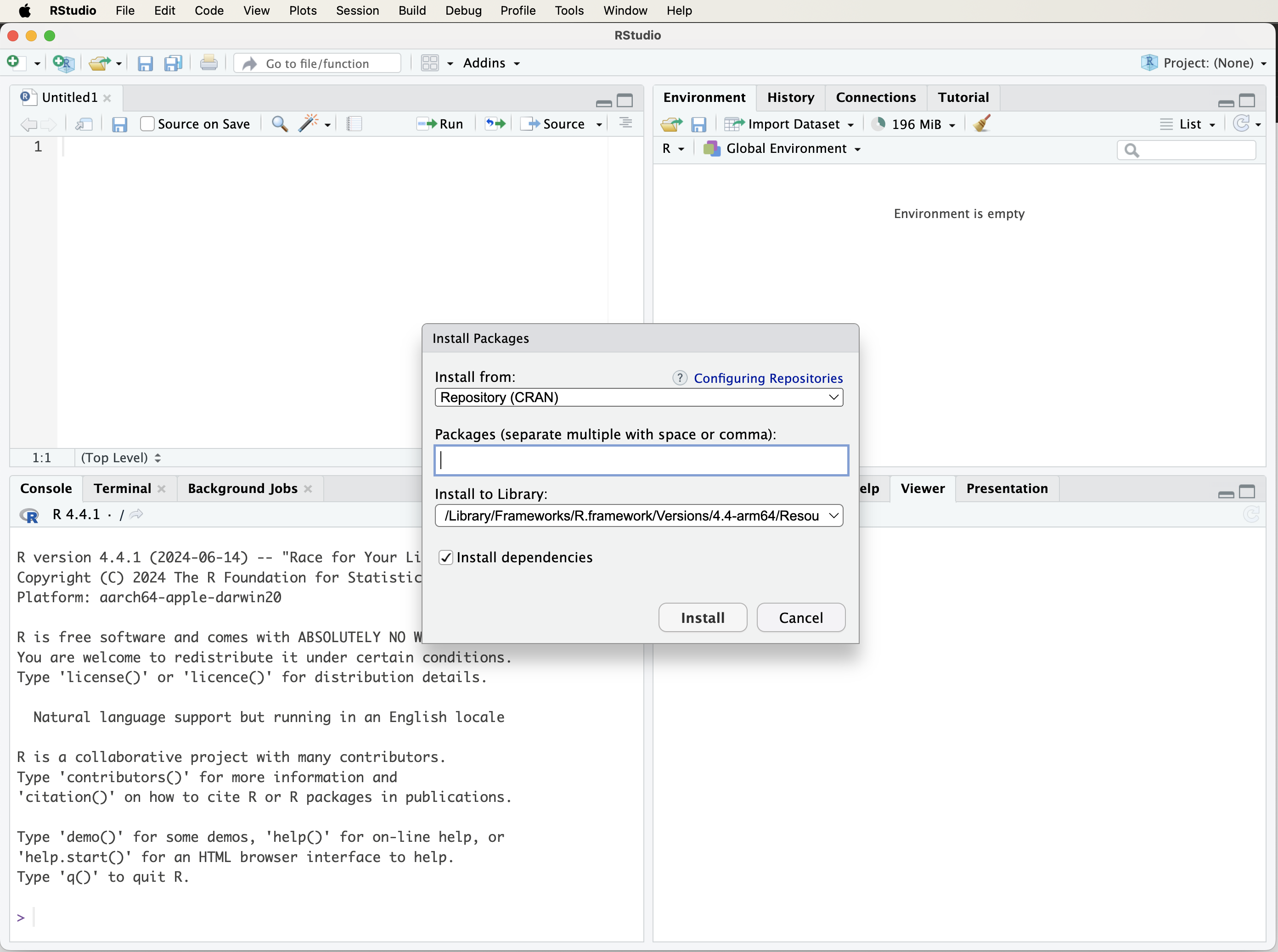
Figure 1.2: A visual guide to installing R packages using the ‘Tools’ tab in RStudio.

The second method is to install packages directly using the install.packages() function. For example, to install the liver package, which provides datasets and functions used throughout this book, enter the following command in the R console:

install.packages("liver")

Press “Enter” to execute the command. R will connect to CRAN and download the package in the correct format for your operating system. If you encounter any issues during installation, ensure you are connected to the internet and that your proxy or firewall is not blocking access to CRAN. The first time you install a package, R may ask you to select a CRAN mirror. Choose one that is geographically close to you for faster downloads.

The install.packages() function also allows for customization, such as installing a package from a local file or a specific repository. To learn more, type the following command in the R console:

?install.packages()

Packages only need to be installed once. After installation, they must be loaded into each new R session using the library() function. We will cover how to load packages in the next section.

1.7 How to Load R Packages

To optimize memory usage, R does not automatically load all installed packages. Instead, you must explicitly load the necessary packages in each new R session. This ensures that only relevant functions and datasets are available, minimizing resource consumption.
To load a package, use the library() or require() function. These functions locate the package on your system and make its functions, datasets, and documentation accessible. For example, to load the liver package, enter the following command in the R console:

library(liver)

Press Enter to execute the command. If an error message appears stating that the package is not found (e.g., "there is no package called 'liver'"), it indicates that the package has not been installed. In such cases, refer to the previous section on installing packages.

Beyond liver, this book utilizes several other R packages, which will be introduced progressively throughout the chapters as needed. However, some R packages contain functions with identical names. For instance, both the liver* and dplyr** packages include a select() function. When multiple packages are loaded, R defaults to using the function from the most recently loaded package.

To explicitly specify which package a function should be sourced from, use the :: operator. This ensures clarity and prevents conflicts. For example, to use the select() function from the liver package, enter:

liver::select()

This approach is particularly useful in complex projects where multiple packages are required, preventing unintended overwrites of functions with the same name.

1.8 Running R Code

R is an interactive language, allowing you to type commands directly into the console and see the results immediately. For example, you can perform basic arithmetic operations such as addition, subtraction, multiplication, and division. To add two numbers, type the following in the R console:

2 + 3
   [1] 5

Press Enter to execute the command. R will compute the sum and display the result. You can also store this result in a variable for later use:

result <- 2 + 3

Here, <- is the assignment operator in R, used to assign values to variables. Some users prefer the = operator (result = 2 + 3), which also works in most cases, but <- remains the recommended convention in R programming.

Variables in R store values for later use, allowing you to perform calculations efficiently. For example, you can multiply result by 4:

result * 4
   [1] 20

R will retrieve the stored value of result and compute the multiplication.

Using Comments in R

Comments are used to explain your code and make it easier to understand. In R, a comment starts with #, and everything following it on that line is ignored by the interpreter.

# Store the sum of 2 and 3 in the variable `result`
result <- 2 + 3

Comments do not affect the execution of your code but are essential for documentation, especially when working on complex projects or collaborating with others.

1.8.1 Functions in R

R provides a rich set of built-in functions to perform specific tasks. A function takes input(s) (arguments), processes them, and returns an output. For example, the c() function creates vectors:

x <- c(1, 2, 3, 4, 5)  # Create a vector

You can then apply functions to this vector. For example, to compute the average of the numbers in x, use the mean() function:

mean(x)  # Calculate the mean of x
   [1] 3

Functions in R follow a simple structure:

function_name(arguments)

Some functions require arguments, while others are optional. To learn more about a function, use ? followed by the function name:

?mean  # or help(mean)

This will open R’s help documentation, providing details about the function’s purpose, usage, arguments, and examples.

Functions are essential in R programming, helping to simplify complex operations and making code more reusable and efficient. As you progress, you will also learn how to write your own functions to automate tasks and improve workflow.

1.9 How to Import Data into R

Before performing any analysis, you first need to load data into R. R can read data from multiple sources, including text files, Excel files, and online datasets. Depending on the file format and data source, you can choose from several methods for importing data into R.

Using RStudio’s Graphical Interface

The easiest way to import data into R is through RStudio’s graphical interface. Click on the Import Dataset button in the top-right panel of RStudio (see Figure 1.3 for a visual guide). This will open a dialog box where you can choose the file type:
- From Text (base) – for CSV or tab-delimited files.
- From Excel – for Microsoft Excel files.
- Other formats are available, depending on installed packages.

After selecting your file, RStudio will display an import settings window (see Figure 1.4). Here, you can adjust column names, data types, and other options. If the first row contains column names, select Yes under the Heading option. Click Import, and the dataset will appear in RStudio’s Environment panel, ready for analysis.

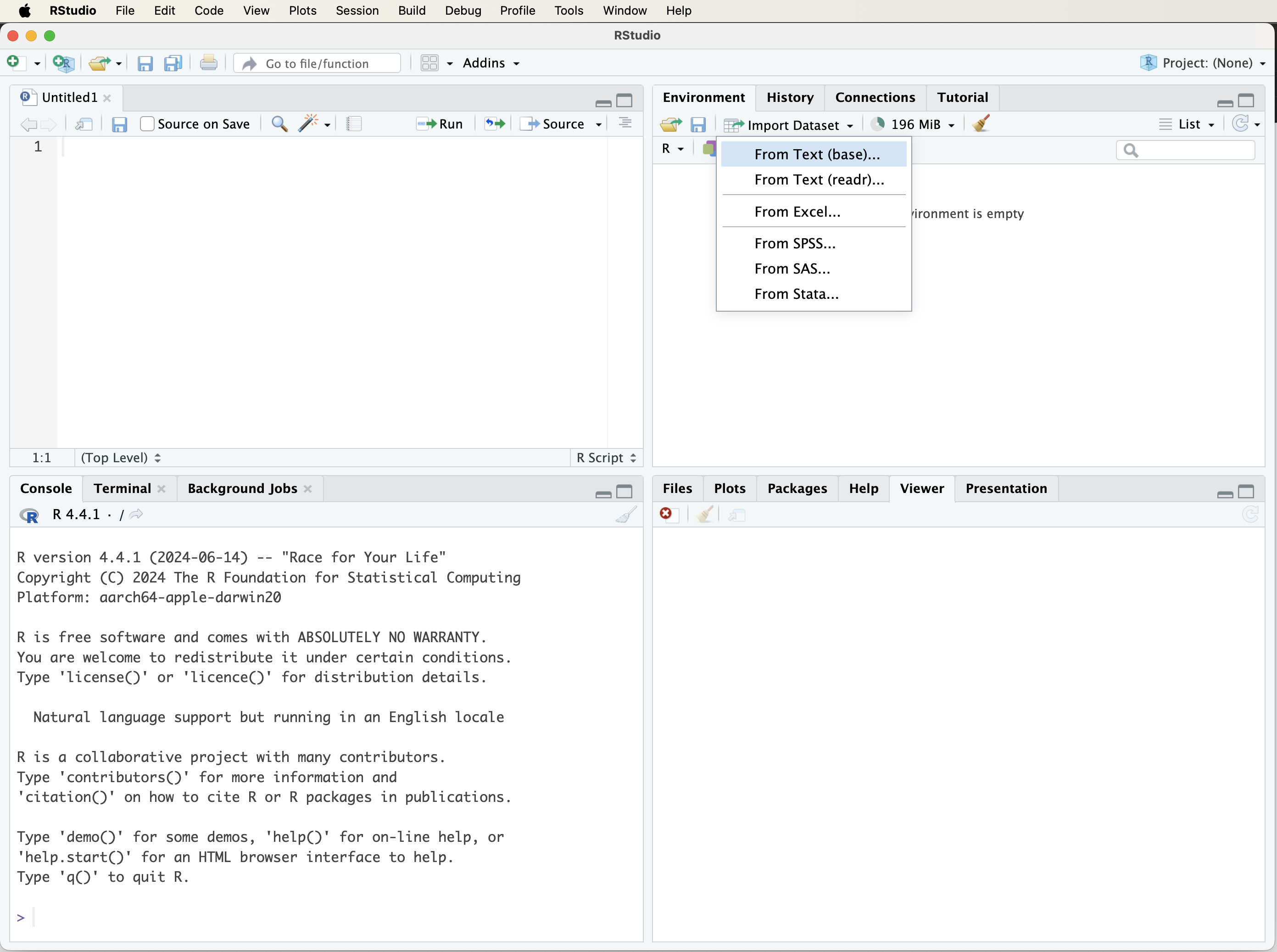
Figure 1.3: A visual guide to loading a dataset into R using the ‘Import Dataset’ tab in RStudio.

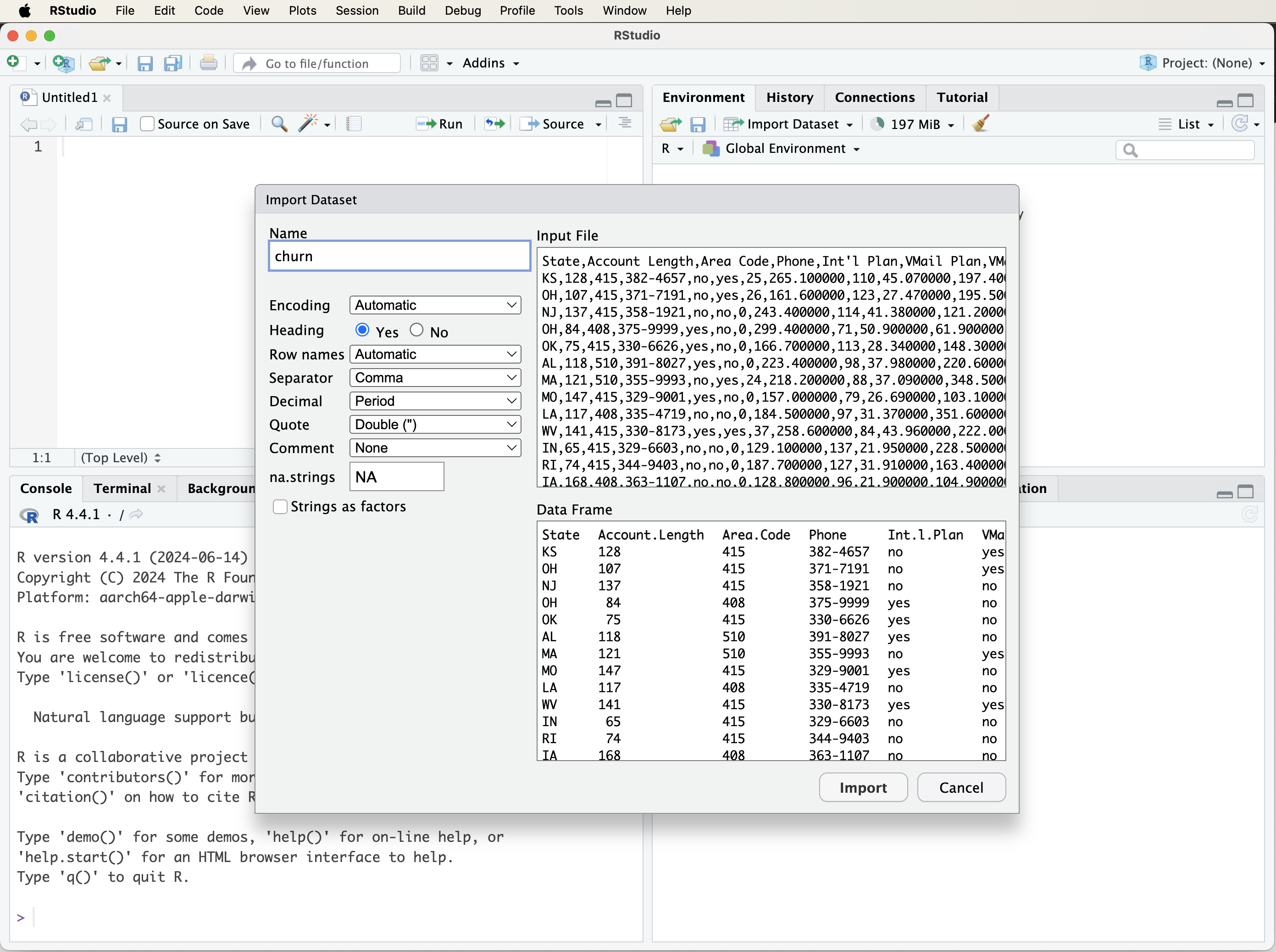
Figure 1.4: A visual guide to customizing the import settings when loading a dataset into R using the ‘Import Dataset’ tab in RStudio.

Using `read.csv()`

You can also import data directly using the read.csv() function, which reads tabular data (such as CSV files) into R as a data frame. If your data file is stored locally, you can load it as follows:

data <- read.csv("path/to/your/file.csv")

Replace "path/to/your/file.csv" with the actual file path. If your file does not contain column names, use:

data <- read.csv("path/to/your/file.csv", header = FALSE)

Setting the Working Directory

By default, R looks for files in the current working directory. If your data is located elsewhere, you can specify the full path in read.csv() or set the working directory.

To check your current working directory:

getwd()

To set a new working directory:

setwd("~/Documents")  # Adjust the path based on your system

Alternatively, in RStudio, go to Session > Set Working Directory > Choose Directory… and select the desired folder.

Using `file.choose()` with `read.csv()`

To interactively select a file instead of typing its path manually, use file.choose():

data <- read.csv(file.choose())

This will open a file selection dialog, making it a convenient option when working with multiple datasets.

Loading Data from Online Sources

R also allows direct import of datasets from web sources. For example, to load a publicly available COVID-19 dataset:

corona_data <- read.csv("https://opendata.ecdc.europa.eu/covid19/casedistribution/csv", na.strings = "", fileEncoding = "UTF-8-BOM")

This approach is useful for accessing open datasets from research institutions or government agencies.

Using `read_excel()` for Excel Files

To import Excel files, use the read_excel() function from the readxl package. First, install and load the package:

install.packages("readxl")

library(readxl)

Then, import the Excel file:

data <- read_excel("path/to/your/file.xlsx")

Unlike read.csv(), read_excel() supports multiple sheets within an Excel file, which can be specified using the sheet argument.
### Loading Data from R Packages {-}

Some datasets are available directly in R packages and do not require importing from an external file. For example, the liver package, developed for this book, contains multiple datasets. To access the churn dataset:

library(liver)
data(churn)

Since many of the datasets used in this book are included in the liver package (see Table 0.1), we will frequently use this package for examples and demonstrations.

This section is well-structured and clearly explains the fundamental data types in R. It is concise and informative, making it accessible to beginners while maintaining a professional tone suitable for a Springer publication. Below are some minor refinements to improve clarity, consistency, and readability.

1.10 Data Types in R

Data in R can take various forms, and correctly identifying these types is essential for effective data manipulation, visualization, and analysis. Each data type has specific properties that determine how R processes it, so understanding them helps avoid errors and ensures accurate results.

Here are the most common data types in R:

Numeric: Represents real numbers, such as 3.14 or -5.67. This type is used for continuous numerical values, like heights, weights, or temperatures.
Integer: Represents whole numbers without decimals, such as 1, 42, or -10. This type is useful for count-based data, such as the number of customers or items sold.
Character: Represents text or string data, such as "Data Science" or "R Programming". This type is commonly used for categorical labels, names, and descriptive values.
Logical: Represents Boolean values: TRUE or FALSE. Logical data is often used in conditional statements and filtering operations.
Factor: Represents categorical data with predefined levels. Factors are commonly used for storing variables such as "Male" or "Female" in a dataset and are particularly useful in statistical modeling.

To check the data type of a variable, use the class() function. For example, to determine the type of the variable result, type:

class(result)
   [1] "numeric"

Press Enter, and R will display the variable’s data type.

Recognizing different data types is essential for choosing the right analytical and visualization techniques. As we will explore in later chapters (e.g., Chapters 4 and 5), numerical and categorical variables require different approaches when performing descriptive statistics, hypothesis testing, and data visualization.

1.11 Data Structures in R

Data structures are fundamental to working with data in R. They define how data is stored and manipulated, which directly impacts the efficiency and accuracy of data analysis. The most commonly used data structures in R are vectors, matrices, data frames, and lists, as illustrated in Figure 1.4.

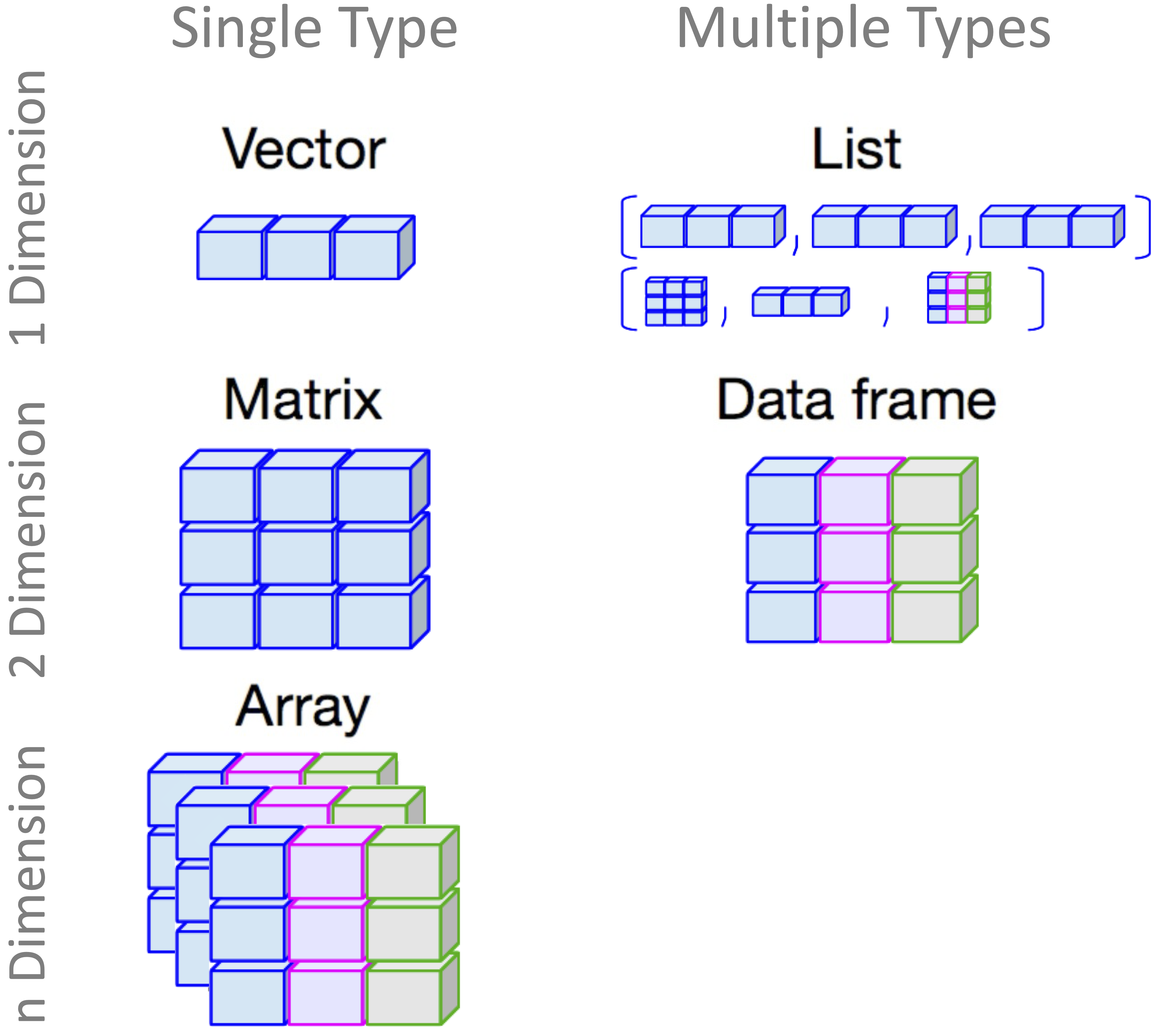
Figure 1.5: A visual guide to different types of data structures in R.

Vectors in R

A vector is the simplest data structure in R. It is a one-dimensional array that holds elements of the same type (numeric, character, or logical). Vectors are the building blocks of other data structures. You can create a vector using the c() function:

# Create a numeric vector
x <- c(1, 2, 0, -3, 5)

# Display the vector
x
   [1]  1  2  0 -3  5

# Check if x is a vector
is.vector(x)
   [1] TRUE

# Check the length of the vector
length(x)
   [1] 5

Here, x is a numeric vector containing five elements. The is.vector() function confirms that x is indeed a vector, while length(x) returns the number of elements in the vector.

Matrices in R

A matrix is a two-dimensional array where all elements must be of the same type. Matrices are useful for mathematical operations and structured numerical data. You can create a matrix using the matrix() function:

# Create a matrix with 2 rows and 3 columns
m <- matrix(c(1, 2, 3, 4, 5, 6), nrow = 2, ncol = 3, byrow = TRUE)

# Display the matrix
m
        [,1] [,2] [,3]
   [1,]    1    2    3
   [2,]    4    5    6

# Check if m is a matrix
is.matrix(m)
   [1] TRUE

# Check the dimensions of the matrix
dim(m)
   [1] 2 3

This matrix m consists of two rows and three columns, filled row-wise. The dim() function returns the dimensions of the matrix. To fill the matrix column-wise, set byrow = FALSE.

Data Frames in R

A data frame is a two-dimensional table where each column can contain a different data type (numeric, character, or logical). This makes data frames ideal for storing tabular data, similar to spreadsheets. You can create a data frame using the data.frame() function:

# Create vectors for student data
student_id <- c(101, 102, 103, 104)
name       <- c("Emma", "Bob", "Alice", "Noah")
age        <- c(20, 21, 19, 22)
grade      <- c("A", "B", "A", "C")

# Create a data frame from the vectors
students_df <- data.frame(student_id, name, age, grade)

# Display the data frame
students_df
     student_id  name age grade
   1        101  Emma  20     A
   2        102   Bob  21     B
   3        103 Alice  19     A
   4        104  Noah  22     C

This data frame students_df consists of four columns: student_id, name, age, and grade. The class() function confirms that an object is a data frame, while is.data.frame() checks its structure.

To inspect the first few rows of a data frame, use the head() function. For example, to display the first six rows of the churn dataset from the liver package:

library(liver)  # Load the liver package
data(churn)     # Load the churn dataset

# Check the structure of the dataset
str(churn)
   'data.frame':    5000 obs. of  20 variables:
    $ state         : Factor w/ 51 levels "AK","AL","AR",..: 17 36 32 36 37 2 20 25 19 50 ...
    $ area.code     : Factor w/ 3 levels "area_code_408",..: 2 2 2 1 2 3 3 2 1 2 ...
    $ account.length: int  128 107 137 84 75 118 121 147 117 141 ...
    $ voice.plan    : Factor w/ 2 levels "yes","no": 1 1 2 2 2 2 1 2 2 1 ...
    $ voice.messages: int  25 26 0 0 0 0 24 0 0 37 ...
    $ intl.plan     : Factor w/ 2 levels "yes","no": 2 2 2 1 1 1 2 1 2 1 ...
    $ intl.mins     : num  10 13.7 12.2 6.6 10.1 6.3 7.5 7.1 8.7 11.2 ...
    $ intl.calls    : int  3 3 5 7 3 6 7 6 4 5 ...
    $ intl.charge   : num  2.7 3.7 3.29 1.78 2.73 1.7 2.03 1.92 2.35 3.02 ...
    $ day.mins      : num  265 162 243 299 167 ...
    $ day.calls     : int  110 123 114 71 113 98 88 79 97 84 ...
    $ day.charge    : num  45.1 27.5 41.4 50.9 28.3 ...
    $ eve.mins      : num  197.4 195.5 121.2 61.9 148.3 ...
    $ eve.calls     : int  99 103 110 88 122 101 108 94 80 111 ...
    $ eve.charge    : num  16.78 16.62 10.3 5.26 12.61 ...
    $ night.mins    : num  245 254 163 197 187 ...
    $ night.calls   : int  91 103 104 89 121 118 118 96 90 97 ...
    $ night.charge  : num  11.01 11.45 7.32 8.86 8.41 ...
    $ customer.calls: int  1 1 0 2 3 0 3 0 1 0 ...
    $ churn         : Factor w/ 2 levels "yes","no": 2 2 2 2 2 2 2 2 2 2 ...

# Display the first six rows
head(churn)
     state     area.code account.length voice.plan voice.messages intl.plan
   1    KS area_code_415            128        yes             25        no
   2    OH area_code_415            107        yes             26        no
   3    NJ area_code_415            137         no              0        no
   4    OH area_code_408             84         no              0       yes
   5    OK area_code_415             75         no              0       yes
   6    AL area_code_510            118         no              0       yes
     intl.mins intl.calls intl.charge day.mins day.calls day.charge eve.mins
   1      10.0          3        2.70    265.1       110      45.07    197.4
   2      13.7          3        3.70    161.6       123      27.47    195.5
   3      12.2          5        3.29    243.4       114      41.38    121.2
   4       6.6          7        1.78    299.4        71      50.90     61.9
   5      10.1          3        2.73    166.7       113      28.34    148.3
   6       6.3          6        1.70    223.4        98      37.98    220.6
     eve.calls eve.charge night.mins night.calls night.charge customer.calls churn
   1        99      16.78      244.7          91        11.01              1    no
   2       103      16.62      254.4         103        11.45              1    no
   3       110      10.30      162.6         104         7.32              0    no
   4        88       5.26      196.9          89         8.86              2    no
   5       122      12.61      186.9         121         8.41              3    no
   6       101      18.75      203.9         118         9.18              0    no

This code loads the liver package, retrieves the churn dataset, and provides an overview of its structure. The str() function is particularly useful for summarizing data frames, as it displays data types and column values.

Lists in R

A list is a flexible data structure that can contain elements of different types, including vectors, matrices, data frames, or even other lists. Lists are useful for storing complex objects in a structured way. You can create a list using the list() function:

# Create a list containing a vector, matrix, and data frame
my_list <- list(vector = x, matrix = m, data_frame = students_df)

# Display the list
my_list
   $vector
   [1]  1  2  0 -3  5
   
   $matrix
        [,1] [,2] [,3]
   [1,]    1    2    3
   [2,]    4    5    6
   
   $data_frame
     student_id  name age grade
   1        101  Emma  20     A
   2        102   Bob  21     B
   3        103 Alice  19     A
   4        104  Noah  22     C

This list my_list stores a vector, a matrix, and a data frame within a single object. Lists allow for efficient organization of heterogeneous data. To explore the structure of a list, use the str() function:

str(my_list)
   List of 3
    $ vector    : num [1:5] 1 2 0 -3 5
    $ matrix    : num [1:2, 1:3] 1 4 2 5 3 6
    $ data_frame:'data.frame':  4 obs. of  4 variables:
     ..$ student_id: num [1:4] 101 102 103 104
     ..$ name      : chr [1:4] "Emma" "Bob" "Alice" "Noah"
     ..$ age       : num [1:4] 20 21 19 22
     ..$ grade     : chr [1:4] "A" "B" "A" "C"

Lists are powerful tools in R, especially for handling nested or hierarchical data. For further exploration, use ?list to access the documentation and additional examples.

1.12 Accessing Records or Variables in R

Once you’ve imported data into R, you can easily access specific records or variables using the $ and [] operators. These tools are essential for extracting data from data frames and lists.

The $ operator allows you to extract a specific column from a data frame or a specific element from a list. For example, to access the name column in the students_df data frame, you would use:

students_df$name
   [1] "Emma"  "Bob"   "Alice" "Noah"

This command retrieves and displays the name column from the students_df data frame.

Similarly, you can use the $ operator to access elements within a list. For example, to access the vector element in the my_list list:

my_list$vector
   [1]  1  2  0 -3  5

This command retrieves and displays the vector element from the my_list list. The $ operator is a straightforward and powerful way to access specific variables or elements within data frames and lists.

Another method for accessing specific records or variables is through the [] operator, which allows you to subset data frames, matrices, and lists based on specific conditions. For example, to extract the first three rows of the students_df data frame, you can use:

students_df[1:3, ]
     student_id  name age grade
   1        101  Emma  20     A
   2        102   Bob  21     B
   3        103 Alice  19     A

This command will display the first three rows of the students_df data frame.

You can also use the [] operator to extract specific columns. For instance, to select the name and grade columns from the students_df data frame:

students_df[, c("name", "grade")]
      name grade
   1  Emma     A
   2   Bob     B
   3 Alice     A
   4  Noah     C

This command retrieves and displays only the name and grade columns from the students_df data frame.

The [] operator is versatile, enabling you to subset data frames, matrices, and lists with precision. Both the $ and [] operators are fundamental tools for data manipulation in R, allowing you to efficiently access and manage the data you need.

1.13 Visualizing Data in R

Data visualization is a powerful tool for exploring and communicating insights from data. It plays a crucial role in exploratory data analysis (EDA), which we will delve into in Chapter 4. As the saying goes, “a picture is worth a thousand words,” and in data science, this is especially true. R provides a broad array of tools for creating high-quality plots and visualizations, allowing you to effectively present your findings.

In R, there are two primary ways to create plots: using base R graphics and using the ggplot2 package. Base R graphics offer a simple and direct way to generate plots, while ggplot2 provides greater flexibility and customization. This book primarily uses ggplot2, as it follows a structured approach based on the grammar of graphics, which breaks down plots into three key components:

Data: The dataset to be visualized, which should be in a data frame format when using ggplot2.
Aesthetics: The visual properties of the data points, such as color, shape, and size.
Geometries: The type of plot to be created, such as scatter plots, bar plots, or line plots.

To create a plot using ggplot2, first install and load the package. Instructions for installing packages are provided in Section 1.6. To load ggplot2, use the following command:

library(ggplot2)

Next, define the data, aesthetics, and geometries for your plot. For example, to create a scatter plot of miles per gallon (mpg) versus horsepower (hp) using the built-in mtcars dataset:

ggplot(data = mtcars) +
  geom_point(mapping = aes(x = mpg, y = hp))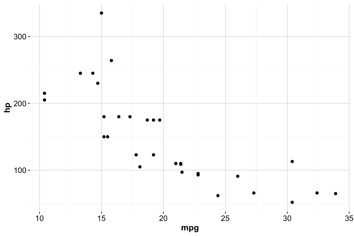

This code initializes the plot with the ggplot() function, specifying the dataset (mtcars). The geom_point() function adds points to the plot, and the aes() function maps mpg to the x-axis and hp to the y-axis.

The general template for creating plots with ggplot2 follows this structure:

ggplot(data = <DATA>) +
  <GEOM_FUNCTION>(mapping = aes(<MAPPINGS>))

Using this template, a variety of visualizations can be created.

Geom Functions in ggplot2

Geom functions determine the type of plot created in ggplot2. Some commonly used geom functions include:

geom_point() for scatter plots
geom_bar() for bar plots
geom_line() for line plots
geom_boxplot() for box plots
geom_histogram() for histograms
geom_density() for density plots
geom_smooth() for adding smoothed conditional means to plots

For example, to create a smoothed line plot of mpg versus hp:

ggplot(data = mtcars) +
  geom_smooth(mapping = aes(x = mpg, y = hp))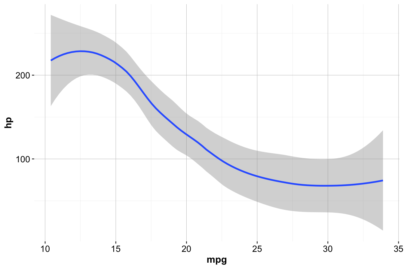

Multiple geom functions can be combined in a single plot. To overlay a scatter plot on the smoothed line:

ggplot(data = mtcars) +
  geom_smooth(mapping = aes(x = mpg, y = hp)) + 
  geom_point(mapping = aes(x = mpg, y = hp))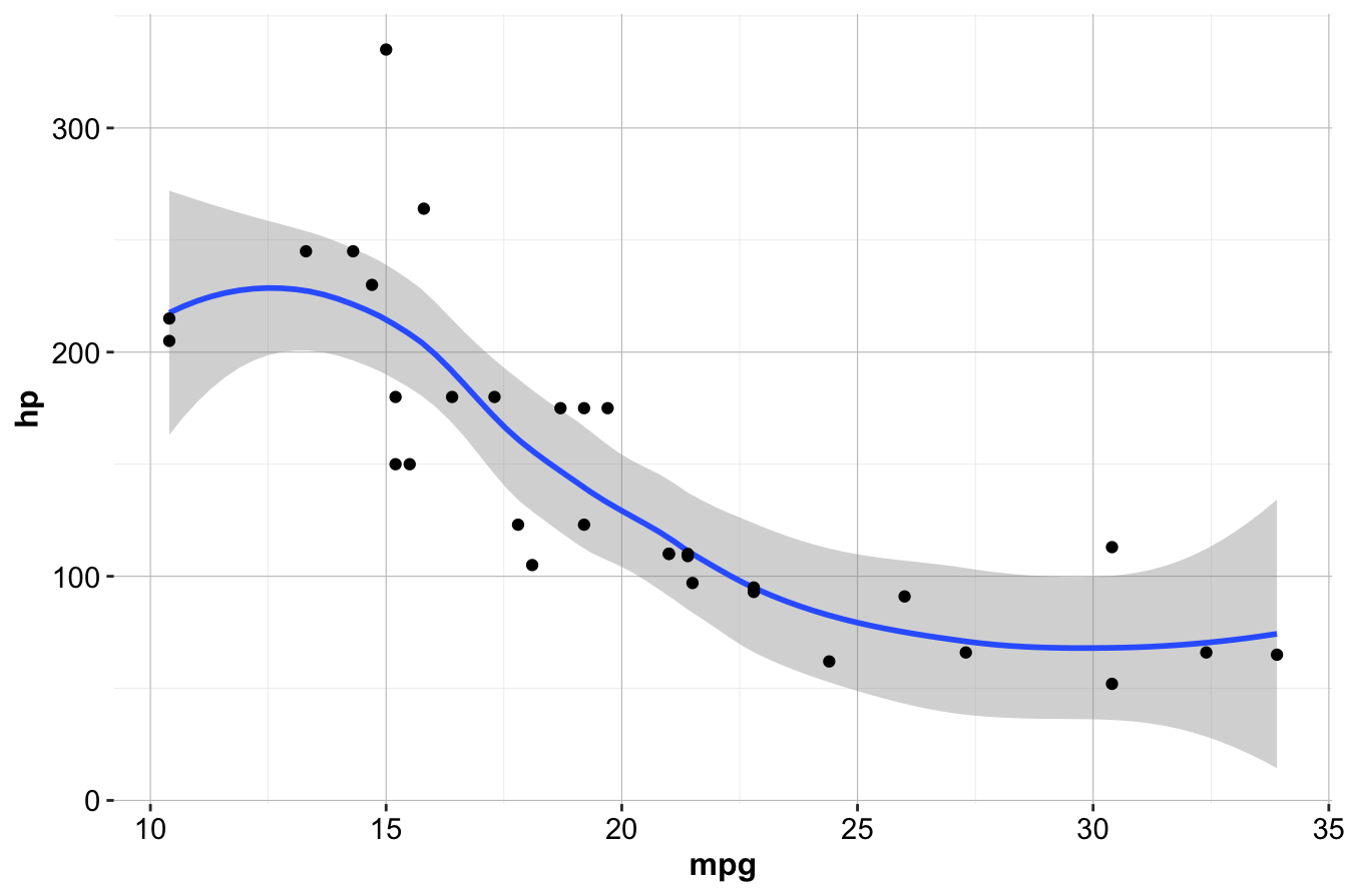

Alternatively, the aes() function can be placed inside ggplot() to streamline the code:

ggplot(data = mtcars, mapping = aes(x = mpg, y = hp)) +
  geom_smooth() + 
  geom_point()

Additional visualization examples can be found in Chapter 4. For a complete list of geom functions, refer to the ggplot2 documentation.

Aesthetics in ggplot2

Aesthetics control the visual properties of data points, such as color, size, and shape. These properties are specified within the aes() function. For example:

ggplot(data = mtcars) +
  geom_point(mapping = aes(x = mpg, y = hp, color = cyl))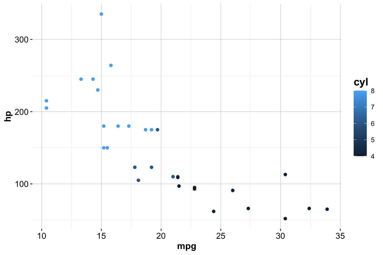

Here, color = cyl maps the color of the points to the number of cylinders (cyl) in the mtcars dataset. ggplot2 automatically assigns a unique color to each category and adds a corresponding legend.

In addition to color, other aesthetics such as size and alpha (transparency) can be used:

# Left plot: using the size aesthetic
ggplot(data = mtcars) +
  geom_point(mapping = aes(x = mpg, y = hp, size = cyl))

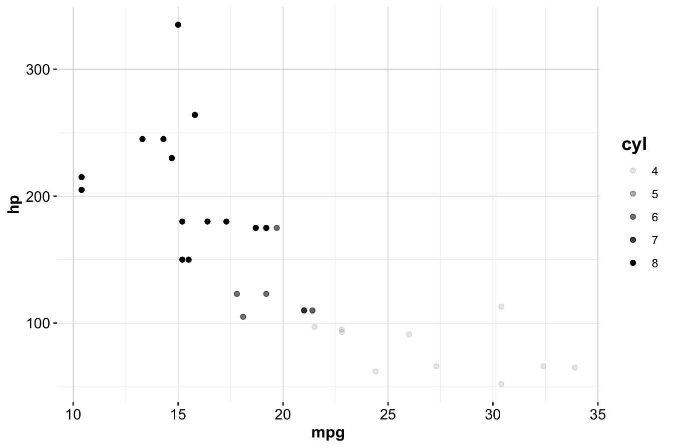
# Right plot: using the alpha aesthetic
ggplot(data = mtcars) +
  geom_point(mapping = aes(x = mpg, y = hp, alpha = cyl))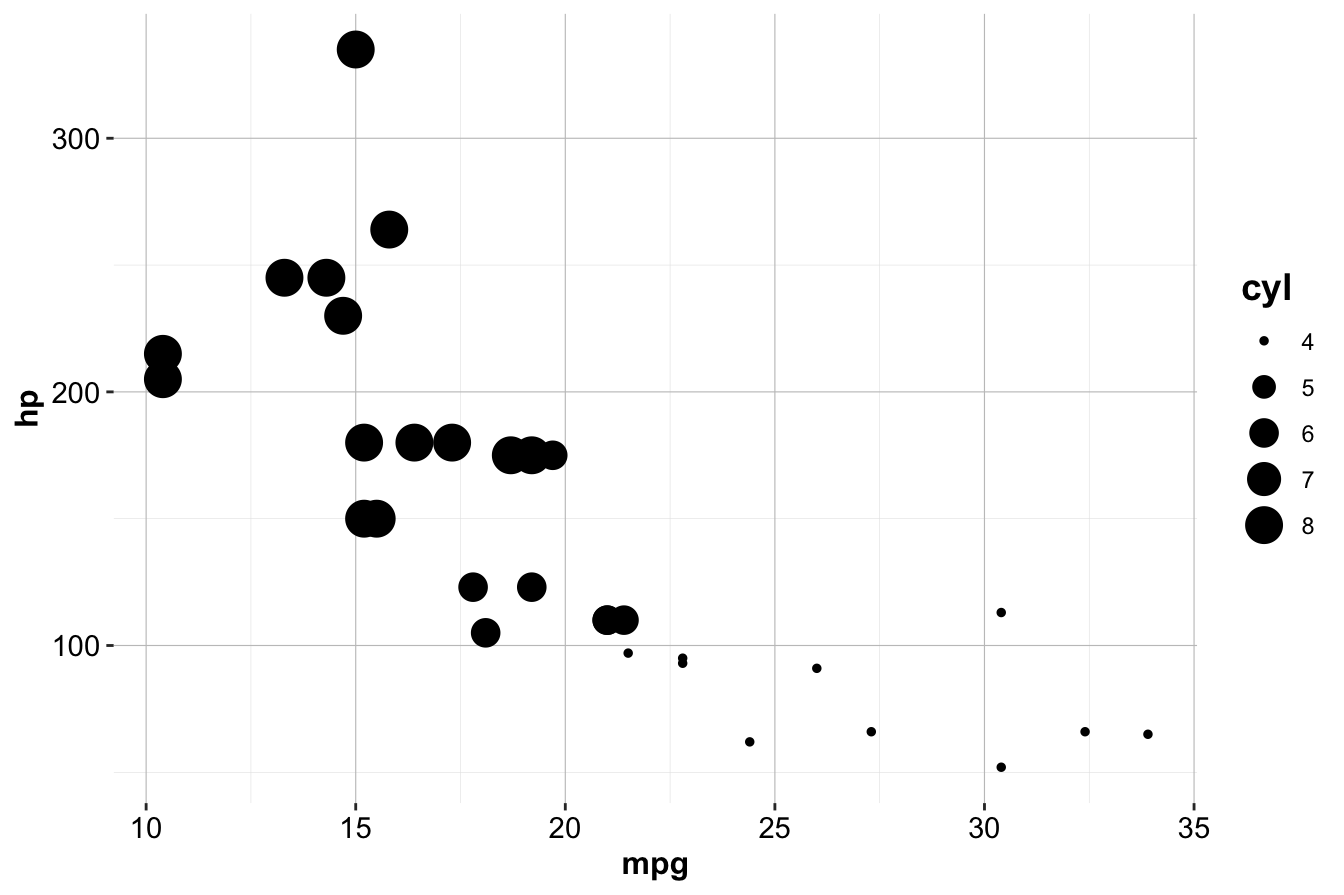

Aesthetics can also be set directly inside geom functions. For example, to make all points blue triangles of size 3:

ggplot(data = mtcars) +
  geom_point(mapping = aes(x = mpg, y = hp), 
             color = "blue", size = 3, shape = 2)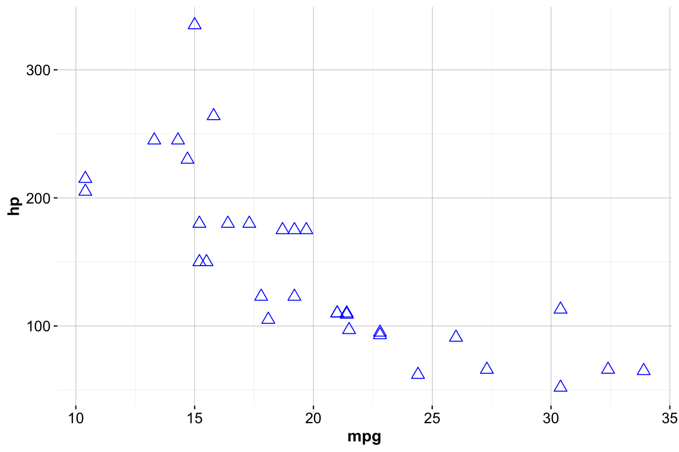

This section introduced the fundamentals of data visualization in R using ggplot2. The next chapters will explore how visualization plays a crucial role in exploratory data analysis (Chapter 4) and how to refine plots for communication and reporting. For more details on visualization techniques, see the ggplot2 documentation. For interactive graphics, consider exploring the plotly package or Shiny for web applications.

1.14 Formula in R

Formulas in R provide a concise and intuitive way to specify relationships between variables for statistical modeling. They are widely used in functions for regression, classification, and machine learning to define how a response variable depends on one or more predictors.

In R, formulas use the tilde symbol ~ to express relationships between variables, where the response variable appears on the left-hand side and predictor variables on the right-hand side. For example, the formula y ~ x specifies that y is modeled as a function of x. When there are multiple predictors, they are separated by +.
For instance, using the diamonds dataset, the formula:

price ~ carat + cut + color

models the price of a diamond based on its carat, cut, and color.

To include all other variables in the dataset as predictors, we can use the shorthand notation:

price ~ .

This approach is particularly useful in large datasets where listing all predictors manually would be impractical.

A formula in R acts as a quoting operator, instructing R to interpret the variables symbolically rather than evaluating them immediately. The variable on the left-hand side of ~ is the dependent variable (or response variable), while the variables on the right-hand side are the independent variables (or predictor variables).

Example 1.1 To illustrate, suppose we want to predict the price of a diamond using a linear regression model. We can pass the formula into the lm() function:

model <- lm(price ~ carat + cut + color, data = diamonds)

Here, the formula price ~ carat + cut + color defines the relationship, and the data argument specifies the dataset to use.

Once defined, formulas can be used in various R functions for statistical modeling and machine learning. As you progress through later chapters, you will encounter formulas in functions for regression, classification, and more (e.g., Chapters 7, 9, and 10). Mastering formula syntax will enable you to efficiently build, customize, and interpret models throughout this book.

1.15 Reporting with R Markdown

Thus far, this book has covered how to interact with R and RStudio for data analysis. This section focuses on an equally important aspect: effectively communicating analytical findings. Data scientists must present results clearly to teams, stakeholders, and clients. Regardless of the depth of an analysis, its impact is limited if it is not communicated effectively. R Markdown facilitates this process by enabling the seamless integration of code, text, and output into dynamic, reproducible reports.

R Markdown allows users to write and execute R code within a document, producing reports, presentations, and dashboards. Unlike traditional notebooks or word processors, R Markdown ensures that text, code, and results remain synchronized as data changes. This book itself is entirely written using R Markdown and generated with the bookdown package, ensuring a fully reproducible and dynamic workflow.

R Markdown documents can be exported into multiple formats, including HTML, PDF, Word, and PowerPoint, making it adaptable to various audiences and reporting needs. Furthermore, it supports the creation of interactive documents using Shiny, allowing users to build web applications that facilitate exploratory data analysis.

To get started, the following resources provide useful references:

R Markdown Cheat Sheet: The R Markdown Cheat Sheet offers a concise reference for creating documents, including syntax, formatting, and output options. It is available in RStudio under Help > Cheatsheets > R Markdown Cheat Sheet.
R Markdown Reference Guide: The R Markdown Reference Guide provides a detailed overview of R Markdown’s features, including document structure and customization.

R Markdown Basics

R Markdown follows a literate programming approach, combining text and executable code in a single document. Unlike word processors where formatting is visible during writing, R Markdown requires compilation to generate the final report. This approach ensures automation, as plots and figures are generated dynamically and inserted into the document. Since the code is embedded, analyses are fully reproducible.

To create an R Markdown document in RStudio:

File > New File > R Markdown

A dialog box will appear, allowing the selection of a document type. For a standard report, choose “Document.” Other options include “Presentation” for slides, “Shiny” for interactive applications, and “From Template” for predefined formats. After selecting the document type, enter a title and author name. The output format can be set to HTML, PDF, or Word; HTML is often recommended for debugging.

R Markdown files use the .Rmd extension, distinguishing them from .R script files. A newly created file contains a template that can be modified with custom text, code, and formatting.

The Header

The header defines metadata such as the document’s title, author, date, and output format. It is enclosed within three dashes (---).

---
title: "An Analysis of Customer Churn"
author: "Reza Mohammadi"
date: "Aug 12, 2024"
output: html_document
---

Title: The document’s title.
Author: The name of the author.
Date: The date of creation.
Output format: The format of the final document (html_document, pdf_document, or word_document).

Additional metadata can be included for customization, such as table of contents options and formatting preferences.

Code Chunks and Inline Code

R Markdown integrates R code within documents using code chunks, which are enclosed in triple backticks (```{r}) followed by the code. For example:


``` r
2 + 3
   [1] 5
```

When compiled, R executes the code and displays the output within the document. Code chunks are used for analysis, visualizations, and modeling. The “Run” button in RStudio allows individual execution of chunks. See Figure 1.6 for a visual guide.

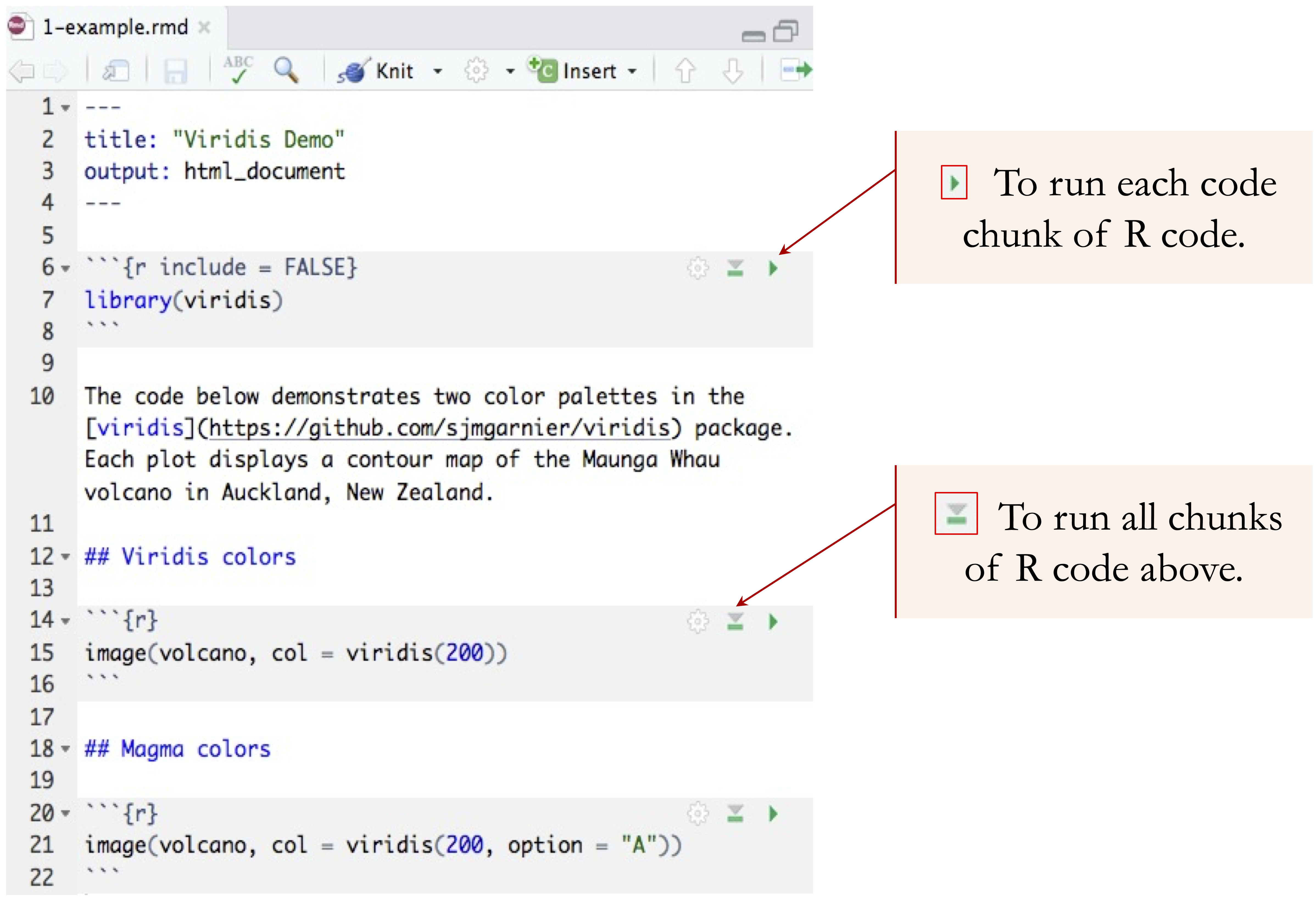
Figure 1.6: Executing a code chunk in R Markdown using the ‘Run’ button in RStudio.

Common chunk options include:

echo = FALSE: Displays output but hides the code.
eval = FALSE: Shows the code but does not execute it.
message = FALSE: Suppresses messages.
warning = FALSE: Suppresses warnings.
error = FALSE: Hides error messages.
include = FALSE: Omits both code and output.

For inline calculations, use backticks and the r keyword:

The factorial of 5 is 120.

This renders dynamically as:

The factorial of 5 is 120.

Styling Text

R Markdown supports various text formatting options:

Headings: Use # for section titles.
Bold: Enclose text in double asterisks (**bold**).
Italic: Use single asterisks (*italic*).
Lists: Use * for bullet points.
Links: [R Markdown website](https://rmarkdown.rstudio.com)
Images: ![Alt text](path/to/image.png)

For mathematical notation, use LaTeX-style equations:

Inline: $y = \beta_0 + \beta_1 x$  
Block: $$ y = \beta_0 + \beta_1 x $$

Mastering R Markdown

For further learning:

Books: R Markdown: The Definitive Guide.
Tutorials: R Markdown website.
Courses: DataCamp R Markdown course.
Forums: RStudio Community.

By leveraging R Markdown, data scientists can produce high-quality, reproducible reports that enhance collaboration and communication.

1.16 Exercises

This section provides hands-on exercises to reinforce your understanding of the fundamental concepts covered in this chapter.

Basic Exercises

Install R and RStudio on your computer.
Use the getwd() function to check your current working directory. Then, change it to a new directory using setwd().
Create a numeric vector named numbers containing the values 5, 10, 15, 20, 25. Then, calculate the mean and standard deviation of the vector.
Create a matrix with 3 rows and 4 columns, filled with numbers from 1 to 12.
Create a data frame containing the following variables:

student_id (integer)
name (character)
score (numeric)
passed (logical, where TRUE means the student passed and FALSE means they failed)
Print the first few rows of the data frame using head().

Install and load the liver and ggplot2 packages in R. If you encounter any errors, check your internet connection and ensure CRAN is accessible.
Load the churn dataset from the liver package and display the first few rows using the head() function.
Report the data types of the variables in the churn dataset using the str() function.
Report the dimensions of the churn dataset using the dim() function.
Report the summary statistics of the variables in the churn dataset using the summary() function.
Create a scatter plot using ggplot2 that visualizes the relationship between day.mins and eve.mins in the churn dataset. Hint: See the code in Section 4.6.
Create a histogram for the day.calls variable in the churn dataset.
Create a boxplot for the day.mins variable in the churn dataset.
Create a boxplot for the day.mins variable in the churn dataset, grouped by the churn variable. Hint: See the code in Section 4.5.
Use the mean() function to compute the mean of the customer.calls variable in the churn dataset. Then, calculate the mean of customer.calls for churner churn == yes.
Create an R Markdown document that includes a title, author, and a small analysis of the churn dataset. Generate an HTML report.

More Challenges Exercise

The following R code generates a simulated dataset with 200 observations. We will use this simulated dataset as a simple toy example in Chapter 7 to explain how k-nearest neighbors algorithm works. This simulated data is for patients with three variables:

Age: Age of the patients as numeric variable with range from 15 to 75 years old.
Ratio: Sodium/Potassium ratio in the patient’s blood as numeric variable. The ratio is generated based on the Type variable.
Type: a factor with three levels: "A", "B", "C" representing the type of drug the patient is taking.

Run the code and report the summary statistics of the data.

# Simulate data for kNN
set.seed(10)

n  = 200         # Number of patients
n1 = 90          # Number of patients with drug A
n2 = 60          # Number of patients with drug B 
n3 = n - n1 - n2 # Number of patients with drug C

# Generate Age variable between 15 and 75
Age = sample(x = 15:75, size = n, replace = TRUE)

# Generate Drug Type variable with three levels
Type = sample(x = c("A", "B", "C"), size = n, replace = TRUE, prob = c(n1, n2, n3))

# Generate Sodium/Potassium Ratio based on Drug Type
Ratio = numeric(n)

Ratio[Type == "A"] = sample(x = 10:40, size = sum(Type == "A"), replace = TRUE)
Ratio[Type == "B"] = sample(x =  5:15, size = sum(Type == "B"), replace = TRUE)
Ratio[Type == "C"] = sample(x =  5:15, size = sum(Type == "C"), replace = TRUE)

# Create a data frame with the generated variables
drug_data = data.frame(Age = Age, Ratio = Ratio, Type = Type)

Visualize the data using the following ggplot2 code:

ggplot(data = drug_data, aes(x = Age, y = Ratio)) +
  geom_point(aes(color = Type, shape = Type)) + 
  labs(title = "Age vs. Sodium/Potassium Ratio", 
       x = "Age", y = "Sodium/Potassium Ratio")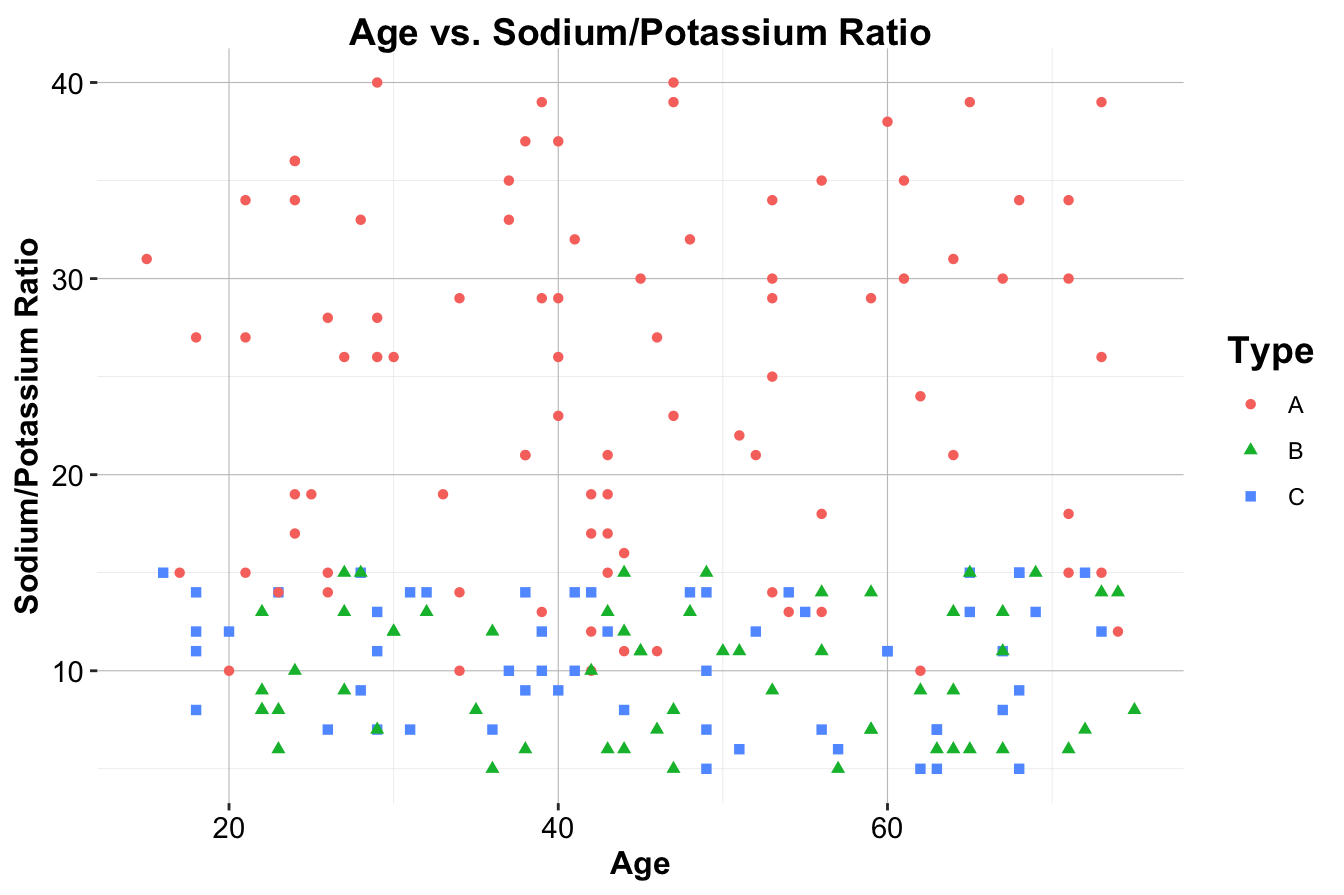

Extend the dataset drug_data by adding a new variable named Outcome, which is a factor with two levels ("Good" and "Bad").

Patients with Type == "A" should have a higher probability of "Good" outcomes.
Patients with Type == "B" and Type == "C" should have a lower probability of "Good" outcomes.
Use sample() with appropriate probabilities to generate the Outcome variable.

Create a new scatter plot using ggplot2 that visualizes the relationship between Age and Ratio, colored by the Outcome variable.
Create a new variable Age_group in the drug_data dataset that categorizes patients into three groups:

“Young” ( $\leq 30$ years old)
“Middle-aged” (31-50 years old)
“Senior” (>50 years old).

Calculate the mean Ratio for each Age_group category in the drug_data dataset.
Create a bar chart using ggplot2 that displays the average Ratio for each Age_group.
Modify the drug_data dataset by adding a Risk_factor variable, calculated as Ratio * Age / 10. Analyze how Risk_factor differs by Type.
Create a histogram of the Risk_factor variable, grouped by Type.
Generate a boxplot to visualize the distribution of Risk_factor across different Outcome categories.

Preface

2 Introduction to Data Science